

220
6 Memristor Circuits: Invariant Manifolds, Coexisting Attractors, Extreme. . .
R
C 1
C 2
v C1
−
+
v C1
−
+
v C2
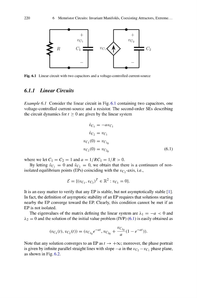
Fig. 6.1 Linear circuit with two capacitors and a voltage-controlled current-source
6.1.1 Linear Circuits
Example 6.1 Consider the linear circuit in Fig. 6.1 containing two capacitors, one
voltage-controlled current-source and a resistor. The second-order SEs describing
the circuit dynamics for t ≥ 0 are given by the linear system
˙
v C 1 = −av C 1
˙
v C 2 = v C 1
v C 1 (0) = v C 1 0
v C 2 (0) = v C 2 0
(6.1)
where we let C 1 = C 2 = 1 and a = 1/RC 1 = 1/R > 0.
By letting ˙
v C 1 = 0 and ˙
v C 2 = 0, we obtain that there is a continuum of nonisolated equilibrium points (EPs) coinciding with the v C 2 -axis, i.e.,
E = {(v C 1 , v C 2 )
T
∈ R
2
: v C 1 = 0}.
It is an easy matter to verify that any EP is stable, but not asymptotically stable [1].
In fact, the definition of asymptotic stability of an EP requires that solutions starting
nearby the EP converge toward the EP. Clearly, this condition cannot be met if an
EP is not isolated.
The eigenvalues of the matrix defining the linear system are λ 1 = −a < 0 and
λ 2 = 0 and the solution of the initial value problem (IVP) (6.1) is easily obtained as
(v C 1 (t), v C 2 (t)) = (v C 1 0 e
−at , v C 2 0 +
v C 1 0
a
(1 − e
−at )).
Note that any solution converges to an EP as t → +∞; moreover, the phase portrait
is given by infinite parallel straight lines with slope −a in the v C 2 −v C 1 phase plane,
as shown in Fig. 6.2.
6 Memristor Circuits: Invariant Manifolds, Coexisting Attractors, Extreme. . .
R
C 1
C 2
v C1
−
+
v C1
−
+
v C2
Fig. 6.1 Linear circuit with two capacitors and a voltage-controlled current-source
6.1.1 Linear Circuits
Example 6.1 Consider the linear circuit in Fig. 6.1 containing two capacitors, one
voltage-controlled current-source and a resistor. The second-order SEs describing
the circuit dynamics for t ≥ 0 are given by the linear system
˙
v C 1 = −av C 1
˙
v C 2 = v C 1
v C 1 (0) = v C 1 0
v C 2 (0) = v C 2 0
(6.1)
where we let C 1 = C 2 = 1 and a = 1/RC 1 = 1/R > 0.
By letting ˙
v C 1 = 0 and ˙
v C 2 = 0, we obtain that there is a continuum of nonisolated equilibrium points (EPs) coinciding with the v C 2 -axis, i.e.,
E = {(v C 1 , v C 2 )
T
∈ R
2
: v C 1 = 0}.
It is an easy matter to verify that any EP is stable, but not asymptotically stable [1].
In fact, the definition of asymptotic stability of an EP requires that solutions starting
nearby the EP converge toward the EP. Clearly, this condition cannot be met if an
EP is not isolated.
The eigenvalues of the matrix defining the linear system are λ 1 = −a < 0 and
λ 2 = 0 and the solution of the initial value problem (IVP) (6.1) is easily obtained as
(v C 1 (t), v C 2 (t)) = (v C 1 0 e
−at , v C 2 0 +
v C 1 0
a
(1 − e
−at )).
Note that any solution converges to an EP as t → +∞; moreover, the phase portrait
is given by infinite parallel straight lines with slope −a in the v C 2 −v C 1 phase plane,
as shown in Fig. 6.2.