

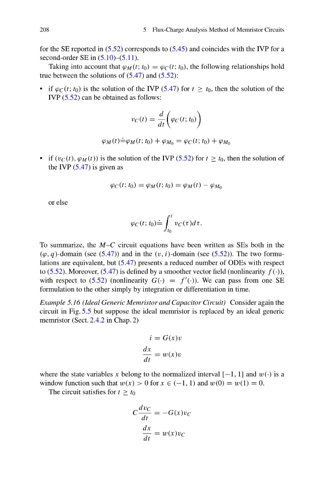
208
5 Flux-Charge Analysis Method of Memristor Circuits
for the SE reported in (5.52) corresponds to (5.45) and coincides with the IVP for a
second-order SE in (5.10)–(5.11).
Taking into account that ϕ M (t; t 0 ) = ϕ C (t; t 0 ), the following relationships hold
true between the solutions of (5.47) and (5.52):
• if ϕ C (t; t 0 ) is the solution of the IVP (5.47) for t ≥ t 0 , then the solution of the
IVP (5.52) can be obtained as follows:
v C (t) =
d
dt
ϕ C (t; t 0 )
ϕ M (t) ˙
=ϕ M (t; t 0 ) + ϕ M 0 = ϕ C (t; t 0 ) + ϕ M 0
• if (v C (t), ϕ M (t)) is the solution of the IVP (5.52) for t ≥ t 0 , then the solution of
the IVP (5.47) is given as
ϕ C (t; t 0 ) = ϕ M (t; t 0 ) = ϕ M (t) − ϕ M 0
or else
ϕ C (t; t 0 ) ˙
=
t
t 0
v C (τ )dτ.
To summarize, the M–C circuit equations have been written as SEs both in the
(ϕ, q)-domain (see (5.47)) and in the (v, i)-domain (see (5.52)). The two formulations are equivalent, but (5.47) presents a reduced number of ODEs with respect
to (5.52). Moreover, (5.47) is defined by a smoother vector field (nonlinearity f (·)),
with respect to (5.52) (nonlinearity G(·) = f (·)). We can pass from one SE
formulation to the other simply by integration or differentiation in time.
Example 5.16 (Ideal Generic Memristor and Capacitor Circuit) Consider again the
circuit in Fig. 5.5 but suppose the ideal memristor is replaced by an ideal generic
memristor (Sect. 2.4.2 in Chap. 2)
i = G(x)v
dx
dt
= w(x)v
where the state variables x belong to the normalized interval [−1, 1] and w(·) is a
window function such that w(x) > 0 for x ∈ (−1, 1) and w(0) = w(1) = 0.
The circuit satisfies for t ≥ t 0
C
dv C
dt
= −G(x)v C
dx
dt
= w(x)v C
5 Flux-Charge Analysis Method of Memristor Circuits
for the SE reported in (5.52) corresponds to (5.45) and coincides with the IVP for a
second-order SE in (5.10)–(5.11).
Taking into account that ϕ M (t; t 0 ) = ϕ C (t; t 0 ), the following relationships hold
true between the solutions of (5.47) and (5.52):
• if ϕ C (t; t 0 ) is the solution of the IVP (5.47) for t ≥ t 0 , then the solution of the
IVP (5.52) can be obtained as follows:
v C (t) =
d
dt
ϕ C (t; t 0 )
ϕ M (t) ˙
=ϕ M (t; t 0 ) + ϕ M 0 = ϕ C (t; t 0 ) + ϕ M 0
• if (v C (t), ϕ M (t)) is the solution of the IVP (5.52) for t ≥ t 0 , then the solution of
the IVP (5.47) is given as
ϕ C (t; t 0 ) = ϕ M (t; t 0 ) = ϕ M (t) − ϕ M 0
or else
ϕ C (t; t 0 ) ˙
=
t
t 0
v C (τ )dτ.
To summarize, the M–C circuit equations have been written as SEs both in the
(ϕ, q)-domain (see (5.47)) and in the (v, i)-domain (see (5.52)). The two formulations are equivalent, but (5.47) presents a reduced number of ODEs with respect
to (5.52). Moreover, (5.47) is defined by a smoother vector field (nonlinearity f (·)),
with respect to (5.52) (nonlinearity G(·) = f (·)). We can pass from one SE
formulation to the other simply by integration or differentiation in time.
Example 5.16 (Ideal Generic Memristor and Capacitor Circuit) Consider again the
circuit in Fig. 5.5 but suppose the ideal memristor is replaced by an ideal generic
memristor (Sect. 2.4.2 in Chap. 2)
i = G(x)v
dx
dt
= w(x)v
where the state variables x belong to the normalized interval [−1, 1] and w(·) is a
window function such that w(x) > 0 for x ∈ (−1, 1) and w(0) = w(1) = 0.
The circuit satisfies for t ≥ t 0
C
dv C
dt
= −G(x)v C
dx
dt
= w(x)v C