

206
5 Flux-Charge Analysis Method of Memristor Circuits
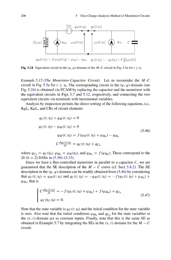
Fig. 5.24 Equivalent circuit in the (ϕ, q)-domain of the M–C circuit in Fig. 5.5a for t ≥ t 0
Example 5.15 (The Memristor-Capacitor Circuit) Let us reconsider the M–C
circuit in Fig. 5.5a for t ≥ t 0 . The corresponding circuit in the (ϕ, q)-domain (see
Fig. 5.24) is obtained via FCAM by replacing the capacitor and the memristor with
the equivalent circuits in Figs. 5.7 and 5.12, respectively, and connecting the two
equivalent circuits via terminals with incremental variables.
Analysis by inspection permits the direct writing of the following equations, i.e.,
KqL, KϕL, and CRs of circuit elements
q C (t; t 0 ) + q M (t; t 0 ) = 0
ϕ C (t; t 0 ) − ϕ M (t; t 0 ) = 0
q M (t; t 0 ) = f (ϕ M (t; t 0 ) + ϕ M 0 ) − q M 0
C
dϕ C (t;t 0 )
dt
= q C (t; t 0 ) + q C 0
(5.46)
where q C 0 = q C (t 0 ), ϕ M 0 = ϕ M (t 0 ), and q M 0 = f (ϕ M 0 ). These correspond to the
2b (b = 2) DAEs in (5.30)–(5.33).
Since we have a flux-controlled memristor in parallel to a capacitor C, we are
guaranteed that the SE description of the M − C exists (cf. Sect. 5.8.2). The SE
description in the (ϕ, q)-domain can be readily obtained from (5.46) by considering
that ϕ C (t; t 0 ) = ϕ M (t; t 0 ) and q C (t; t 0 ) = −q M (t; t 0 ) = −f (ϕ C (t; t 0 ) + ϕ M 0 ) +
q M 0 , that is
⎧
⎨
⎩
C
dϕ C (t;t 0 )
dt
= −f (ϕ C (t; t 0 ) + ϕ M 0 ) + f (ϕ M 0 ) + q C 0
ϕ C (t 0 ; t 0 ) = 0.
(5.47)
Note that the state variable is ϕ C (t; t 0 ) and the initial condition for the state variable
is zero. Also note that the initial conditions ϕ M 0 and q C 0 for the state variables in
the (v, i)-domain act as constant inputs. Finally, note that this is the same SE as
obtained in Example 5.7 by integrating the SEs in the (v, i)-domain for the M − C
circuit.
5 Flux-Charge Analysis Method of Memristor Circuits
Fig. 5.24 Equivalent circuit in the (ϕ, q)-domain of the M–C circuit in Fig. 5.5a for t ≥ t 0
Example 5.15 (The Memristor-Capacitor Circuit) Let us reconsider the M–C
circuit in Fig. 5.5a for t ≥ t 0 . The corresponding circuit in the (ϕ, q)-domain (see
Fig. 5.24) is obtained via FCAM by replacing the capacitor and the memristor with
the equivalent circuits in Figs. 5.7 and 5.12, respectively, and connecting the two
equivalent circuits via terminals with incremental variables.
Analysis by inspection permits the direct writing of the following equations, i.e.,
KqL, KϕL, and CRs of circuit elements
q C (t; t 0 ) + q M (t; t 0 ) = 0
ϕ C (t; t 0 ) − ϕ M (t; t 0 ) = 0
q M (t; t 0 ) = f (ϕ M (t; t 0 ) + ϕ M 0 ) − q M 0
C
dϕ C (t;t 0 )
dt
= q C (t; t 0 ) + q C 0
(5.46)
where q C 0 = q C (t 0 ), ϕ M 0 = ϕ M (t 0 ), and q M 0 = f (ϕ M 0 ). These correspond to the
2b (b = 2) DAEs in (5.30)–(5.33).
Since we have a flux-controlled memristor in parallel to a capacitor C, we are
guaranteed that the SE description of the M − C exists (cf. Sect. 5.8.2). The SE
description in the (ϕ, q)-domain can be readily obtained from (5.46) by considering
that ϕ C (t; t 0 ) = ϕ M (t; t 0 ) and q C (t; t 0 ) = −q M (t; t 0 ) = −f (ϕ C (t; t 0 ) + ϕ M 0 ) +
q M 0 , that is
⎧
⎨
⎩
C
dϕ C (t;t 0 )
dt
= −f (ϕ C (t; t 0 ) + ϕ M 0 ) + f (ϕ M 0 ) + q C 0
ϕ C (t 0 ; t 0 ) = 0.
(5.47)
Note that the state variable is ϕ C (t; t 0 ) and the initial condition for the state variable
is zero. Also note that the initial conditions ϕ M 0 and q C 0 for the state variables in
the (v, i)-domain act as constant inputs. Finally, note that this is the same SE as
obtained in Example 5.7 by integrating the SEs in the (v, i)-domain for the M − C
circuit.