

158
4 Nonlinear Dynamics and Bifurcations in Autonomous RLC Circuits
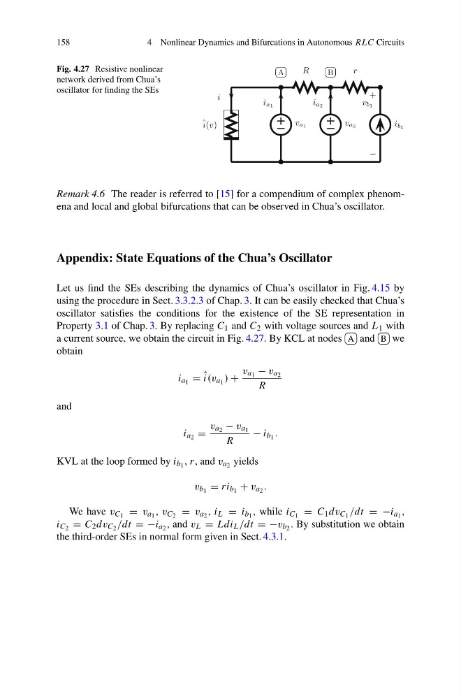
Fig. 4.27 Resistive nonlinear
network derived from Chua’s
oscillator for finding the SEs
ˆ i(v)
v a1
R
v a2
r
i b1
−
+
v b1
i
i a1
i a2
A
B
Remark 4.6 The reader is referred to [15] for a compendium of complex phenomena and local and global bifurcations that can be observed in Chua’s oscillator.
Appendix: State Equations of the Chua’s Oscillator
Let us find the SEs describing the dynamics of Chua’s oscillator in Fig. 4.15 by
using the procedure in Sect. 3.3.2.3 of Chap. 3. It can be easily checked that Chua’s
oscillator satisfies the conditions for the existence of the SE representation in
Property 3.1 of Chap. 3. By replacing C 1 and C 2 with voltage sources and L 1 with
a current source, we obtain the circuit in Fig. 4.27. By KCL at nodes A and B we
obtain
i a 1 = ˆ
i(v a 1 ) +
v a 1 − v a 2
R
and
i a 2 =
v a 2 − v a 1
R
− i b 1 .
KVL at the loop formed by i b 1 , r, and v a 2 yields
v b 1 = ri b 1 + v a 2 .
We have v C 1 = v a 1 , v C 2 = v a 2 , i L = i b 1 , while i C 1 = C 1 dv C 1 /dt = −i a 1 ,
i C 2 = C 2 dv C 2 /dt = −i a 2 , and v L = Ldi L /dt = −v b 2 . By substitution we obtain
the third-order SEs in normal form given in Sect. 4.3.1.
4 Nonlinear Dynamics and Bifurcations in Autonomous RLC Circuits
Fig. 4.27 Resistive nonlinear
network derived from Chua’s
oscillator for finding the SEs
ˆ i(v)
v a1
R
v a2
r
i b1
−
+
v b1
i
i a1
i a2
A
B
Remark 4.6 The reader is referred to [15] for a compendium of complex phenomena and local and global bifurcations that can be observed in Chua’s oscillator.
Appendix: State Equations of the Chua’s Oscillator
Let us find the SEs describing the dynamics of Chua’s oscillator in Fig. 4.15 by
using the procedure in Sect. 3.3.2.3 of Chap. 3. It can be easily checked that Chua’s
oscillator satisfies the conditions for the existence of the SE representation in
Property 3.1 of Chap. 3. By replacing C 1 and C 2 with voltage sources and L 1 with
a current source, we obtain the circuit in Fig. 4.27. By KCL at nodes A and B we
obtain
i a 1 = ˆ
i(v a 1 ) +
v a 1 − v a 2
R
and
i a 2 =
v a 2 − v a 1
R
− i b 1 .
KVL at the loop formed by i b 1 , r, and v a 2 yields
v b 1 = ri b 1 + v a 2 .
We have v C 1 = v a 1 , v C 2 = v a 2 , i L = i b 1 , while i C 1 = C 1 dv C 1 /dt = −i a 1 ,
i C 2 = C 2 dv C 2 /dt = −i a 2 , and v L = Ldi L /dt = −v b 2 . By substitution we obtain
the third-order SEs in normal form given in Sect. 4.3.1.