

4.4 Bifurcations of Equilibrium Points and Periodic Orbits
151
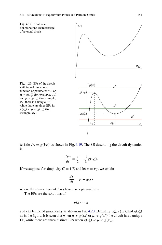
Fig. 4.19 Nonlinear
nonmonotone characteristic
of a tunnel diode
Fig. 4.20 EPs of the circuit
with tunnel diode as a
function of parameter μ. For
μ < g(x
0 ) (for example, μ a )
and μ > g(x 0 ) (for example,
μ c ) there is a unique EP,
while there are three EPs for
g(x
0 ) < μ < g(x 0 ) (for
example, μ b )
teristic I D = g(V D ) as shown in Fig. 4.19. The SE describing the circuit dynamics
is
dv C
dt
=
I
C
−
1
C
g(v C ).
If we suppose for simplicity C = 1 F, and let x = v C , we obtain
dx
dt
= μ − g(x)
where the source current I is chosen as a parameter μ.
The EPs are the solutions of
g(x) = μ
and can be found graphically as shown in Fig. 4.20. Define x 0 , x
0 , g(x 0 ), and g(x
0 )
as in the figure. It is seen that when μ > g(x 0 ) or μ < g(x
0 ) the circuit has a unique
EP, while there are three distinct EPs when g(x
0 ) < μ < g(x 0 ).
151
Fig. 4.19 Nonlinear
nonmonotone characteristic
of a tunnel diode
Fig. 4.20 EPs of the circuit
with tunnel diode as a
function of parameter μ. For
μ < g(x
0 ) (for example, μ a )
and μ > g(x 0 ) (for example,
μ c ) there is a unique EP,
while there are three EPs for
g(x
0 ) < μ < g(x 0 ) (for
example, μ b )
teristic I D = g(V D ) as shown in Fig. 4.19. The SE describing the circuit dynamics
is
dv C
dt
=
I
C
−
1
C
g(v C ).
If we suppose for simplicity C = 1 F, and let x = v C , we obtain
dx
dt
= μ − g(x)
where the source current I is chosen as a parameter μ.
The EPs are the solutions of
g(x) = μ
and can be found graphically as shown in Fig. 4.20. Define x 0 , x
0 , g(x 0 ), and g(x
0 )
as in the figure. It is seen that when μ > g(x 0 ) or μ < g(x
0 ) the circuit has a unique
EP, while there are three distinct EPs when g(x
0 ) < μ < g(x 0 ).