

3.3 State Equations
127
q C = ˆ
q C (v C )
and the inductors are current-controlled, i.e., they satisfy the CRs
ϕ L = ˆ
ϕ L (i L ).
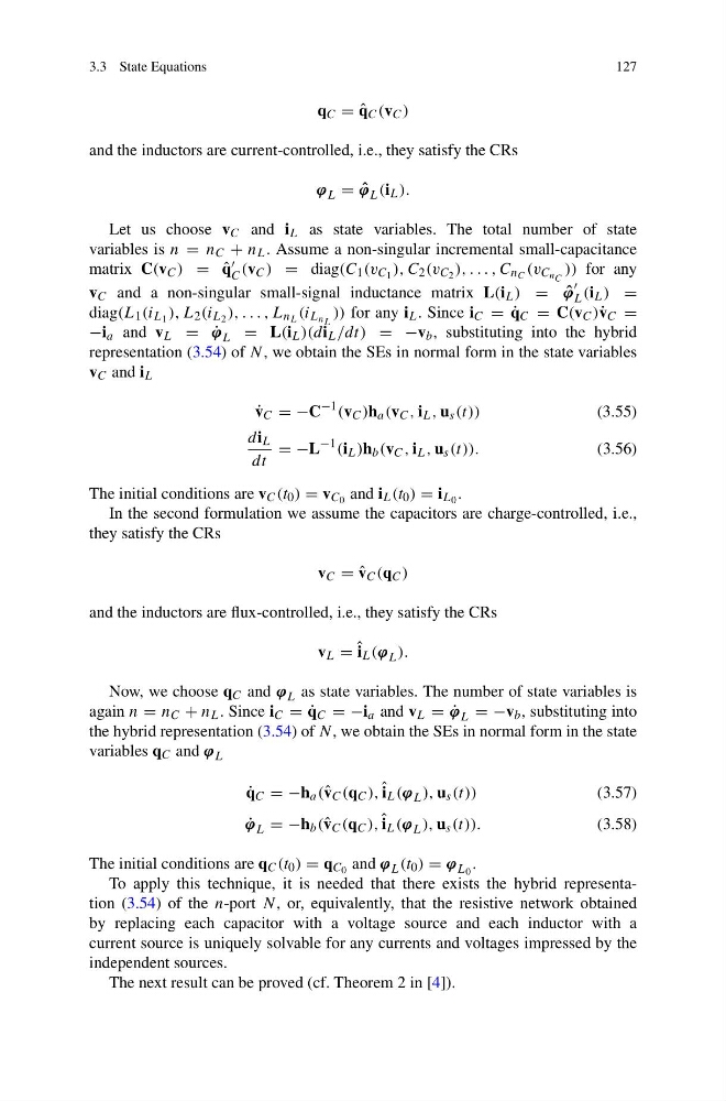
Let us choose v C and i L as state variables. The total number of state
variables is n = n C + n L . Assume a non-singular incremental small-capacitance
matrix C(v C ) = ˆ
q
C (v C ) = diag(C 1 (v C 1 ), C 2 (v C 2 ), . . . , C n C (v C n C )) for any
v C and a non-singular small-signal inductance matrix L(i L ) = ˆ
ϕ
L (i L ) =
diag(L 1 (i L 1 ), L 2 (i L 2 ), . . . , L n L (i L n L )) for any i L . Since i C = ˙
q C = C(v C )˙ v C =
−i a and v L = ˙
ϕ L = L(i L )(di L /dt) = −v b , substituting into the hybrid
representation (3.54) of N , we obtain the SEs in normal form in the state variables
v C and i L
˙
v C = −C
−1 (v C )h a (v C , i L , u s (t))
(3.55)
di L
dt
= −L
−1 (i L )h b (v C , i L , u s (t)).
(3.56)
The initial conditions are v C (t 0 ) = v C 0 and i L (t 0 ) = i L 0 .
In the second formulation we assume the capacitors are charge-controlled, i.e.,
they satisfy the CRs
v C = ˆ
v C (q C )
and the inductors are flux-controlled, i.e., they satisfy the CRs
v L = ˆ i L (ϕ L ).
Now, we choose q C and ϕ L as state variables. The number of state variables is
again n = n C + n L . Since i C = ˙
q C = −i a and v L = ˙
ϕ L = −v b , substituting into
the hybrid representation (3.54) of N, we obtain the SEs in normal form in the state
variables q C and ϕ L
˙
q C = −h a (ˆ v C (q C ), ˆ i L (ϕ L ), u s (t))
(3.57)
˙
ϕ L = −h b (ˆ v C (q C ), ˆ i L (ϕ L ), u s (t)).
(3.58)
The initial conditions are q C (t 0 ) = q C 0 and ϕ L (t 0 ) = ϕ L 0 .
To apply this technique, it is needed that there exists the hybrid representation (3.54) of the n-port N, or, equivalently, that the resistive network obtained
by replacing each capacitor with a voltage source and each inductor with a
current source is uniquely solvable for any currents and voltages impressed by the
independent sources.
The next result can be proved (cf. Theorem 2 in [4]).
127
q C = ˆ
q C (v C )
and the inductors are current-controlled, i.e., they satisfy the CRs
ϕ L = ˆ
ϕ L (i L ).
Let us choose v C and i L as state variables. The total number of state
variables is n = n C + n L . Assume a non-singular incremental small-capacitance
matrix C(v C ) = ˆ
q
C (v C ) = diag(C 1 (v C 1 ), C 2 (v C 2 ), . . . , C n C (v C n C )) for any
v C and a non-singular small-signal inductance matrix L(i L ) = ˆ
ϕ
L (i L ) =
diag(L 1 (i L 1 ), L 2 (i L 2 ), . . . , L n L (i L n L )) for any i L . Since i C = ˙
q C = C(v C )˙ v C =
−i a and v L = ˙
ϕ L = L(i L )(di L /dt) = −v b , substituting into the hybrid
representation (3.54) of N , we obtain the SEs in normal form in the state variables
v C and i L
˙
v C = −C
−1 (v C )h a (v C , i L , u s (t))
(3.55)
di L
dt
= −L
−1 (i L )h b (v C , i L , u s (t)).
(3.56)
The initial conditions are v C (t 0 ) = v C 0 and i L (t 0 ) = i L 0 .
In the second formulation we assume the capacitors are charge-controlled, i.e.,
they satisfy the CRs
v C = ˆ
v C (q C )
and the inductors are flux-controlled, i.e., they satisfy the CRs
v L = ˆ i L (ϕ L ).
Now, we choose q C and ϕ L as state variables. The number of state variables is
again n = n C + n L . Since i C = ˙
q C = −i a and v L = ˙
ϕ L = −v b , substituting into
the hybrid representation (3.54) of N, we obtain the SEs in normal form in the state
variables q C and ϕ L
˙
q C = −h a (ˆ v C (q C ), ˆ i L (ϕ L ), u s (t))
(3.57)
˙
ϕ L = −h b (ˆ v C (q C ), ˆ i L (ϕ L ), u s (t)).
(3.58)
The initial conditions are q C (t 0 ) = q C 0 and ϕ L (t 0 ) = ϕ L 0 .
To apply this technique, it is needed that there exists the hybrid representation (3.54) of the n-port N, or, equivalently, that the resistive network obtained
by replacing each capacitor with a voltage source and each inductor with a
current source is uniquely solvable for any currents and voltages impressed by the
independent sources.
The next result can be proved (cf. Theorem 2 in [4]).