

124
3 RLC Networks Equations and Analysis Methods
C 1
1 Ω
R 1
i R1
+
−
v R1
R 2
i R2
+
−
v R2
1 A
L 2
+
−
v 1
i1
+
−
v 2
i2
(a)
v 1
1 Ω
R 1
i R1
+
−
v R1
R 2
i R2
+
−
v R2
1 A
i 2
+
−
v 1
i1
+
−
v 2
i2
C
(b)
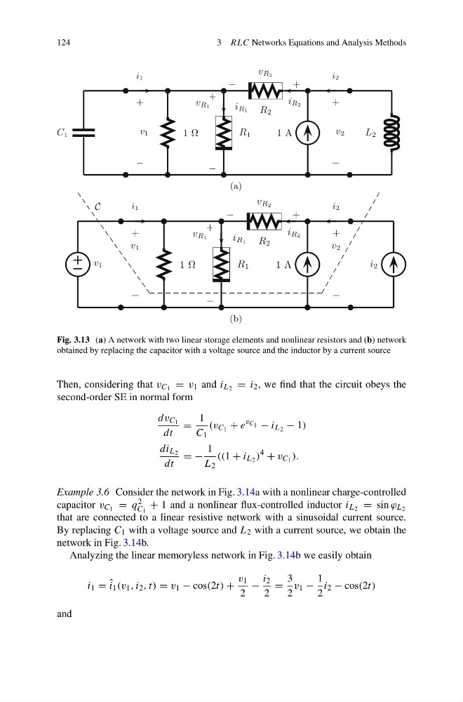
Fig. 3.13 (a) A network with two linear storage elements and nonlinear resistors and (b) network
obtained by replacing the capacitor with a voltage source and the inductor by a current source
Then, considering that v C 1 = v 1 and i L 2 = i 2 , we find that the circuit obeys the
second-order SE in normal form
dv C 1
dt
=
1
C 1
(v C 1 + e
v C 1 − i L 2 − 1)
di L 2
dt
= −
1
L 2
((1 + i L 2 )
4
+ v C 1 ).
Example 3.6 Consider the network in Fig. 3.14a with a nonlinear charge-controlled
capacitor v C 1 = q 2
C 1
+ 1 and a nonlinear flux-controlled inductor i L 2 = sin ϕ L 2
that are connected to a linear resistive network with a sinusoidal current source.
By replacing C 1 with a voltage source and L 2 with a current source, we obtain the
network in Fig. 3.14b.
Analyzing the linear memoryless network in Fig. 3.14b we easily obtain
i 1 = ˆ
i 1 (v 1 , i 2 , t) = v 1 − cos(2t) +
v 1
2
−
i 2
2
=
3
2
v 1 −
1
2
i 2 − cos(2t)
and
3 RLC Networks Equations and Analysis Methods
C 1
1 Ω
R 1
i R1
+
−
v R1
R 2
i R2
+
−
v R2
1 A
L 2
+
−
v 1
i1
+
−
v 2
i2
(a)
v 1
1 Ω
R 1
i R1
+
−
v R1
R 2
i R2
+
−
v R2
1 A
i 2
+
−
v 1
i1
+
−
v 2
i2
C
(b)
Fig. 3.13 (a) A network with two linear storage elements and nonlinear resistors and (b) network
obtained by replacing the capacitor with a voltage source and the inductor by a current source
Then, considering that v C 1 = v 1 and i L 2 = i 2 , we find that the circuit obeys the
second-order SE in normal form
dv C 1
dt
=
1
C 1
(v C 1 + e
v C 1 − i L 2 − 1)
di L 2
dt
= −
1
L 2
((1 + i L 2 )
4
+ v C 1 ).
Example 3.6 Consider the network in Fig. 3.14a with a nonlinear charge-controlled
capacitor v C 1 = q 2
C 1
+ 1 and a nonlinear flux-controlled inductor i L 2 = sin ϕ L 2
that are connected to a linear resistive network with a sinusoidal current source.
By replacing C 1 with a voltage source and L 2 with a current source, we obtain the
network in Fig. 3.14b.
Analyzing the linear memoryless network in Fig. 3.14b we easily obtain
i 1 = ˆ
i 1 (v 1 , i 2 , t) = v 1 − cos(2t) +
v 1
2
−
i 2
2
=
3
2
v 1 −
1
2
i 2 − cos(2t)
and