

6.5 Modeling Tissues
127
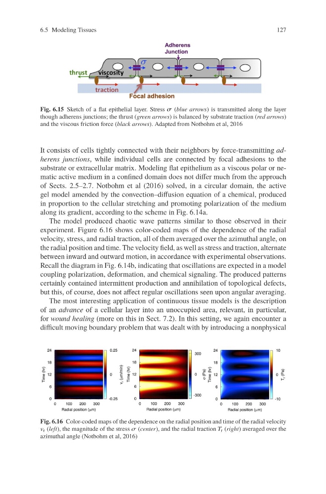
Fig. 6.15 Sketch of a flat epithelial layer. Stress σ (blue arrows) is transmitted along the layer
though adherens junctions; the thrust (green arrows) is balanced by substrate traction (red arrows)
and the viscous friction force (black arrows). Adapted from Notbohm et al, 2016
It consists of cells tightly connected with their neighbors by force-transmitting adherens junctions, while individual cells are connected by focal adhesions to the
substrate or extracellular matrix. Modeling flat epithelium as a viscous polar or nematic active medium in a confined domain does not differ much from the approach
of Sects. 2.5–2.7. Notbohm et al (2016) solved, in a circular domain, the active
gel model amended by the convection–diffusion equation of a chemical, produced
in proportion to the cellular stretching and promoting polarization of the medium
along its gradient, according to the scheme in Fig. 6.14a.
The model produced chaotic wave patterns similar to those observed in their
experiment. Figure 6.16 shows color-coded maps of the dependence of the radial
velocity, stress, and radial traction, all of them averaged over the azimuthal angle, on
the radial position and time. The velocity field, as well as stress and traction, alternate
between inward and outward motion, in accordance with experimental observations.
Recall the diagram in Fig. 6.14b, indicating that oscillations are expected in a model
coupling polarization, deformation, and chemical signaling. The produced patterns
certainly contained intermittent production and annihilation of topological defects,
but this, of course, does not affect regular oscillations seen upon angular averaging.
The most interesting application of continuous tissue models is the description
of an advance of a cellular layer into an unoccupied area, relevant, in particular,
for wound healing (more on this in Sect. 7.2). In this setting, we again encounter a
difficult moving boundary problem that was dealt with by introducing a nonphysical
Fig. 6.16 Color-coded maps of the dependence on the radial position and time of the radial velocity
v r (left), the magnitude of the stress σ (center), and the radial traction T r (right) averaged over the
azimuthal angle (Notbohm et al, 2016)
127
Fig. 6.15 Sketch of a flat epithelial layer. Stress σ (blue arrows) is transmitted along the layer
though adherens junctions; the thrust (green arrows) is balanced by substrate traction (red arrows)
and the viscous friction force (black arrows). Adapted from Notbohm et al, 2016
It consists of cells tightly connected with their neighbors by force-transmitting adherens junctions, while individual cells are connected by focal adhesions to the
substrate or extracellular matrix. Modeling flat epithelium as a viscous polar or nematic active medium in a confined domain does not differ much from the approach
of Sects. 2.5–2.7. Notbohm et al (2016) solved, in a circular domain, the active
gel model amended by the convection–diffusion equation of a chemical, produced
in proportion to the cellular stretching and promoting polarization of the medium
along its gradient, according to the scheme in Fig. 6.14a.
The model produced chaotic wave patterns similar to those observed in their
experiment. Figure 6.16 shows color-coded maps of the dependence of the radial
velocity, stress, and radial traction, all of them averaged over the azimuthal angle, on
the radial position and time. The velocity field, as well as stress and traction, alternate
between inward and outward motion, in accordance with experimental observations.
Recall the diagram in Fig. 6.14b, indicating that oscillations are expected in a model
coupling polarization, deformation, and chemical signaling. The produced patterns
certainly contained intermittent production and annihilation of topological defects,
but this, of course, does not affect regular oscillations seen upon angular averaging.
The most interesting application of continuous tissue models is the description
of an advance of a cellular layer into an unoccupied area, relevant, in particular,
for wound healing (more on this in Sect. 7.2). In this setting, we again encounter a
difficult moving boundary problem that was dealt with by introducing a nonphysical
Fig. 6.16 Color-coded maps of the dependence on the radial position and time of the radial velocity
v r (left), the magnitude of the stress σ (center), and the radial traction T r (right) averaged over the
azimuthal angle (Notbohm et al, 2016)