

outcomes with their counterparts in the physical world (i.e. standards, measured
data, empirical graphs).
There are different ways to represent variables and relationships behind a dynamical model in Coach, including (a) the stock and flow mode (graphical representation) and (b) text-based modes, using equations or a textual representation. In this
chapter, we confined ourselves to graphical modelling with a stock and flow
representation of variables and relationships among these variables. This was
because the stock and flow representations stimulate pupils to focus on qualitative
relationships (theoretical world) and connections of these to the realistic situation
(physical world) rather than mathematical equations or programming syntaxes.
12.4.3.2 Examples of Coach Modelling Activities
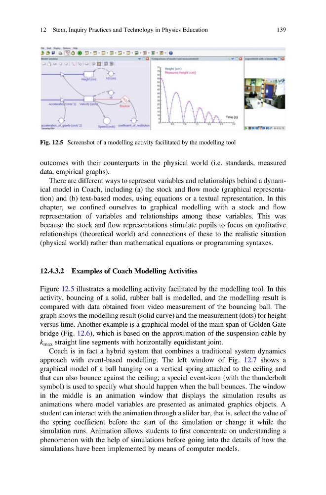
Figure 12.5 illustrates a modelling activity facilitated by the modelling tool. In this
activity, bouncing of a solid, rubber ball is modelled, and the modelling result is
compared with data obtained from video measurement of the bouncing ball. The
graph shows the modelling result (solid curve) and the measurement (dots) for height
versus time. Another example is a graphical model of the main span of Golden Gate
bridge (Fig. 12.6), which is based on the approximation of the suspension cable by
k max straight line segments with horizontally equidistant joint.
Coach is in fact a hybrid system that combines a traditional system dynamics
approach with event-based modelling. The left window of Fig. 12.7 shows a
graphical model of a ball hanging on a vertical spring attached to the ceiling and
that can also bounce against the ceiling; a special event-icon (with the thunderbolt
symbol) is used to specify what should happen when the ball bounces. The window
in the middle is an animation window that displays the simulation results as
animations where model variables are presented as animated graphics objects. A
student can interact with the animation through a slider bar, that is, select the value of
the spring coefficient before the start of the simulation or change it while the
simulation runs. Animation allows students to first concentrate on understanding a
phenomenon with the help of simulations before going into the details of how the
simulations have been implemented by means of computer models.
Fig. 12.5 Screenshot of a modelling activity facilitated by the modelling tool
12 Stem, Inquiry Practices and Technology in Physics Education
139
data, empirical graphs).
There are different ways to represent variables and relationships behind a dynamical model in Coach, including (a) the stock and flow mode (graphical representation) and (b) text-based modes, using equations or a textual representation. In this
chapter, we confined ourselves to graphical modelling with a stock and flow
representation of variables and relationships among these variables. This was
because the stock and flow representations stimulate pupils to focus on qualitative
relationships (theoretical world) and connections of these to the realistic situation
(physical world) rather than mathematical equations or programming syntaxes.
12.4.3.2 Examples of Coach Modelling Activities
Figure 12.5 illustrates a modelling activity facilitated by the modelling tool. In this
activity, bouncing of a solid, rubber ball is modelled, and the modelling result is
compared with data obtained from video measurement of the bouncing ball. The
graph shows the modelling result (solid curve) and the measurement (dots) for height
versus time. Another example is a graphical model of the main span of Golden Gate
bridge (Fig. 12.6), which is based on the approximation of the suspension cable by
k max straight line segments with horizontally equidistant joint.
Coach is in fact a hybrid system that combines a traditional system dynamics
approach with event-based modelling. The left window of Fig. 12.7 shows a
graphical model of a ball hanging on a vertical spring attached to the ceiling and
that can also bounce against the ceiling; a special event-icon (with the thunderbolt
symbol) is used to specify what should happen when the ball bounces. The window
in the middle is an animation window that displays the simulation results as
animations where model variables are presented as animated graphics objects. A
student can interact with the animation through a slider bar, that is, select the value of
the spring coefficient before the start of the simulation or change it while the
simulation runs. Animation allows students to first concentrate on understanding a
phenomenon with the help of simulations before going into the details of how the
simulations have been implemented by means of computer models.
Fig. 12.5 Screenshot of a modelling activity facilitated by the modelling tool
12 Stem, Inquiry Practices and Technology in Physics Education
139