

U k ðr; QÞ ¼
X
k
a k ðtÞU
a
k ðtÞ:
ð3:2:18Þ
Therefore, the probabilities of detecting a system in different adiabatic states of
the fast subsystem, i.e., the coefficients a k ðtÞ
j
j
2 depend on time in this case. It means
that the slow subsystem makes transitions between states defined by quantum
numbers k, i.e., between different PECs. Such transitions are called nonadiabatic. To
calculate these probabilities is to describe nonadiabatic transitions. If the coefficients
a k ðtÞ = const 6 ¼ f(t), then the adiabatic approximation is quite applicable.
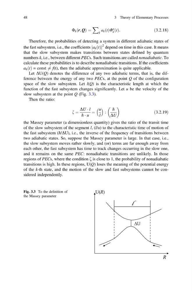
Let DU(Q) denotes the difference of any two adiabatic terms, that is, the difference between the energy of any two PECs, at the point Q of the configuration
space of the slow subsystem. Let l(Q) is the characteristic length at which the
function of the fast subsystem changes significantly. Let u be the velocity of the
slow subsystem at the point Q (Fig. 3.3).
Then the ratio:
f ¼
DU Á l
h Á u
¼
u
l
:
h
DU
ð3:2:19Þ
the Massey parameter (a dimensionless quantity) gives the ratio of the transit time
of the slow subsystem of the segment l, (l/u) to the characteristic time of motion of
the fast subsystem (ħ/DU), i.e., the inverse of the frequency of transitions between
two adiabatic states. So, suppose the Massey parameter is large. In that case, i.e.,
the slow subsystem moves rather slowly, and (or) terms are far enough away from
each other, the fast subsystem has time to track changes occurring in the slow one,
and it remains on the same PEC: nonadiabatic transitions are unlikely. In those
regions of PECs, where the condition f is close to 1, the probability of nonadiabatic
transitions is high. In these regions, U(Q) loses the meaning of the potential energy
of the k-th state, and the motion of the slow and fast subsystems cannot be considered independently.
Fig. 3.3 To the definition of
the Massey parameter
48
3 Theory of Elementary Processes
X
k
a k ðtÞU
a
k ðtÞ:
ð3:2:18Þ
Therefore, the probabilities of detecting a system in different adiabatic states of
the fast subsystem, i.e., the coefficients a k ðtÞ
j
j
2 depend on time in this case. It means
that the slow subsystem makes transitions between states defined by quantum
numbers k, i.e., between different PECs. Such transitions are called nonadiabatic. To
calculate these probabilities is to describe nonadiabatic transitions. If the coefficients
a k ðtÞ = const 6 ¼ f(t), then the adiabatic approximation is quite applicable.
Let DU(Q) denotes the difference of any two adiabatic terms, that is, the difference between the energy of any two PECs, at the point Q of the configuration
space of the slow subsystem. Let l(Q) is the characteristic length at which the
function of the fast subsystem changes significantly. Let u be the velocity of the
slow subsystem at the point Q (Fig. 3.3).
Then the ratio:
f ¼
DU Á l
h Á u
¼
u
l
:
h
DU
ð3:2:19Þ
the Massey parameter (a dimensionless quantity) gives the ratio of the transit time
of the slow subsystem of the segment l, (l/u) to the characteristic time of motion of
the fast subsystem (ħ/DU), i.e., the inverse of the frequency of transitions between
two adiabatic states. So, suppose the Massey parameter is large. In that case, i.e.,
the slow subsystem moves rather slowly, and (or) terms are far enough away from
each other, the fast subsystem has time to track changes occurring in the slow one,
and it remains on the same PEC: nonadiabatic transitions are unlikely. In those
regions of PECs, where the condition f is close to 1, the probability of nonadiabatic
transitions is high. In these regions, U(Q) loses the meaning of the potential energy
of the k-th state, and the motion of the slow and fast subsystems cannot be considered independently.
Fig. 3.3 To the definition of
the Massey parameter
48
3 Theory of Elementary Processes