

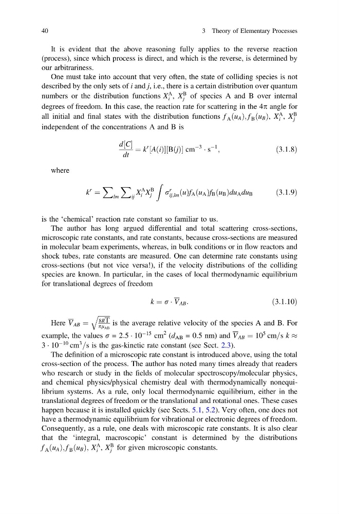
It is evident that the above reasoning fully applies to the reverse reaction
(process), since which process is direct, and which is the reverse, is determined by
our arbitrariness.
One must take into account that very often, the state of colliding species is not
described by the only sets of i and j, i.e., there is a certain distribution over quantum
numbers or the distribution functions X
A
i , X
B
j of species A and B over internal
degrees of freedom. In this case, the reaction rate for scattering in the 4p angle for
all initial and final states with the distribution functions f A u A
ð Þ; f B ðu B Þ, X
A
i , X
B
j
independent of the concentrations A and B is
d½C
dt
¼ k
r
½AðiÞ½BðjÞ cm
À3
Á s
À1
;
ð3:1:8Þ
where
k
r
¼
X
lm
X
ij
X
A
i X
B
j
Z
r
r
ij;lm ðuÞf A u A
ð Þf B u B
ð Þdu A du B
ð3:1:9Þ
is the ‘chemical’ reaction rate constant so familiar to us.
The author has long argued differential and total scattering cross-sections,
microscopic rate constants, and rate constants, because cross-sections are measured
in molecular beam experiments, whereas, in bulk conditions or in flow reactors and
shock tubes, rate constants are measured. One can determine rate constants using
cross-sections (but not vice versa!), if the velocity distributions of the colliding
species are known. In particular, in the cases of local thermodynamic equilibrium
for translational degrees of freedom
k ¼ r Á V AB :
ð3:1:10Þ
Here V AB ¼
ffiffiffiffiffiffiffi ffi
8RT
pl AB
q
is the average relative velocity of the species A and B. For
example, the values r = 2:5 Á 10
À15 cm
2 (d AB = 0.5 nm) and V AB ¼ 10
5 cm=s k %
3 Á 10
À10 cm
3
=s is the gas-kinetic rate constant (see Sect. 2.3).
The definition of a microscopic rate constant is introduced above, using the total
cross-section of the process. The author has noted many times already that readers
who research or study in the fields of molecular spectroscopy/molecular physics,
and chemical physics/physical chemistry deal with thermodynamically nonequilibrium systems. As a rule, only local thermodynamic equilibrium, either in the
translational degrees of freedom or the translational and rotational ones. These cases
happen because it is installed quickly (see Sects. 5.1, 5.2). Very often, one does not
have a thermodynamic equilibrium for vibrational or electronic degrees of freedom.
Consequently, as a rule, one deals with microscopic rate constants. It is also clear
that the ‘integral, macroscopic’ constant is determined by the distributions
f A u A
ð Þ; f B u B
ð Þ; X
A
i , X
B
j for given microscopic constants.
40
3 Theory of Elementary Processes
(process), since which process is direct, and which is the reverse, is determined by
our arbitrariness.
One must take into account that very often, the state of colliding species is not
described by the only sets of i and j, i.e., there is a certain distribution over quantum
numbers or the distribution functions X
A
i , X
B
j of species A and B over internal
degrees of freedom. In this case, the reaction rate for scattering in the 4p angle for
all initial and final states with the distribution functions f A u A
ð Þ; f B ðu B Þ, X
A
i , X
B
j
independent of the concentrations A and B is
d½C
dt
¼ k
r
½AðiÞ½BðjÞ cm
À3
Á s
À1
;
ð3:1:8Þ
where
k
r
¼
X
lm
X
ij
X
A
i X
B
j
Z
r
r
ij;lm ðuÞf A u A
ð Þf B u B
ð Þdu A du B
ð3:1:9Þ
is the ‘chemical’ reaction rate constant so familiar to us.
The author has long argued differential and total scattering cross-sections,
microscopic rate constants, and rate constants, because cross-sections are measured
in molecular beam experiments, whereas, in bulk conditions or in flow reactors and
shock tubes, rate constants are measured. One can determine rate constants using
cross-sections (but not vice versa!), if the velocity distributions of the colliding
species are known. In particular, in the cases of local thermodynamic equilibrium
for translational degrees of freedom
k ¼ r Á V AB :
ð3:1:10Þ
Here V AB ¼
ffiffiffiffiffiffiffi ffi
8RT
pl AB
q
is the average relative velocity of the species A and B. For
example, the values r = 2:5 Á 10
À15 cm
2 (d AB = 0.5 nm) and V AB ¼ 10
5 cm=s k %
3 Á 10
À10 cm
3
=s is the gas-kinetic rate constant (see Sect. 2.3).
The definition of a microscopic rate constant is introduced above, using the total
cross-section of the process. The author has noted many times already that readers
who research or study in the fields of molecular spectroscopy/molecular physics,
and chemical physics/physical chemistry deal with thermodynamically nonequilibrium systems. As a rule, only local thermodynamic equilibrium, either in the
translational degrees of freedom or the translational and rotational ones. These cases
happen because it is installed quickly (see Sects. 5.1, 5.2). Very often, one does not
have a thermodynamic equilibrium for vibrational or electronic degrees of freedom.
Consequently, as a rule, one deals with microscopic rate constants. It is also clear
that the ‘integral, macroscopic’ constant is determined by the distributions
f A u A
ð Þ; f B u B
ð Þ; X
A
i , X
B
j for given microscopic constants.
40
3 Theory of Elementary Processes