

1. Obtain the reciprocal lattice net of the given (direct) lattice as per the procedure
given in section 2.2.
2. Construct a Wigner–Seitz (W–S) unit cell in the resulting reciprocal lattice
according to the set procedure given in section 2.1. This will represent the first
B-Z corresponding to the given direct lattice.
Since the exact nature of the region in the form of line, plane or space within the
first B-Z (according to lattice dimension) is governed by the diffraction condition,
therefore let us start with Bragg’s diffraction condition to understand the construction of B-Z in 1-D, 2-D and 3D lattices, one by one.
(a) One-Dimensional Lattice
We know that the general form of Bragg’s diffraction condition is given by
G
2
þ 2k : G ¼ 0
ð2:1Þ
However for a 1-D lattice, the components of the reciprocal lattice vector G and
the wave vector k are given by
G ¼
2p
a
^ i n x and k ¼ ^ i k x
Substituting these values in Eq. 2.1, we obtain
2p
a
^ i n x
! 2
þ 2 ^ i k x :
2p
a
^ i n x ¼ 0
or
4p
2
a 2 n
2
x þ
4p
a
n x k x ¼ 0
or
k x ¼ À
p
a
n x
ð2:2Þ
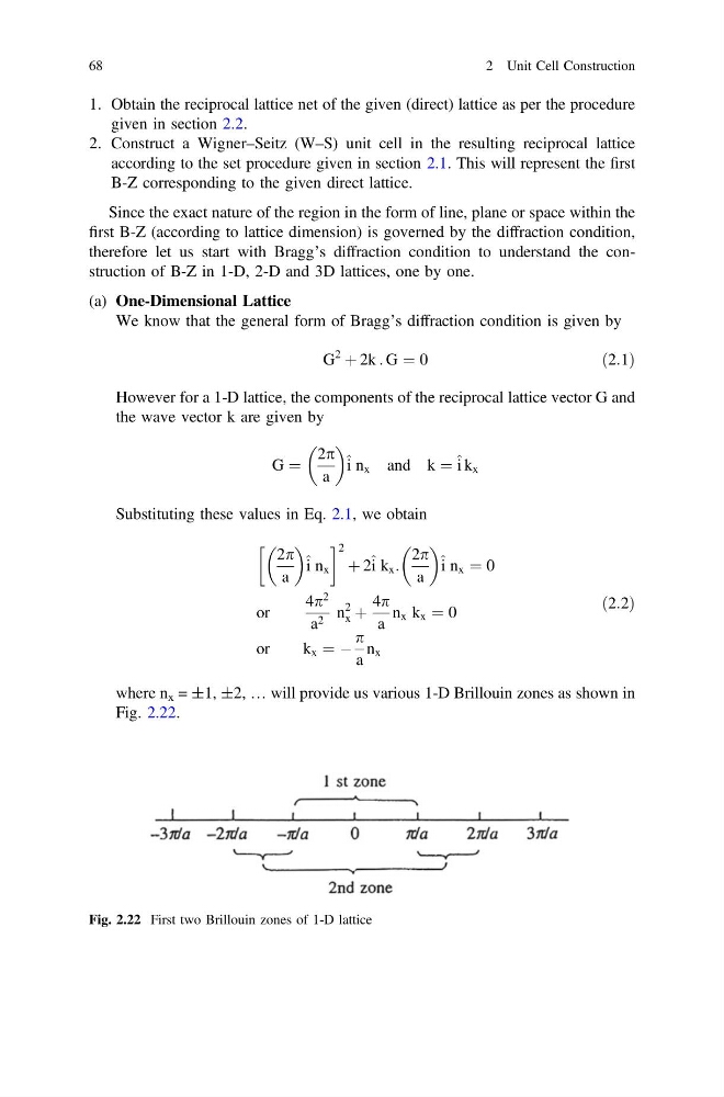
where n x = ±1, ±2, … will provide us various 1-D Brillouin zones as shown in
Fig. 2.22.
Fig. 2.22 First two Brillouin zones of 1-D lattice
68
2 Unit Cell Construction
given in section 2.2.
2. Construct a Wigner–Seitz (W–S) unit cell in the resulting reciprocal lattice
according to the set procedure given in section 2.1. This will represent the first
B-Z corresponding to the given direct lattice.
Since the exact nature of the region in the form of line, plane or space within the
first B-Z (according to lattice dimension) is governed by the diffraction condition,
therefore let us start with Bragg’s diffraction condition to understand the construction of B-Z in 1-D, 2-D and 3D lattices, one by one.
(a) One-Dimensional Lattice
We know that the general form of Bragg’s diffraction condition is given by
G
2
þ 2k : G ¼ 0
ð2:1Þ
However for a 1-D lattice, the components of the reciprocal lattice vector G and
the wave vector k are given by
G ¼
2p
a
^ i n x and k ¼ ^ i k x
Substituting these values in Eq. 2.1, we obtain
2p
a
^ i n x
! 2
þ 2 ^ i k x :
2p
a
^ i n x ¼ 0
or
4p
2
a 2 n
2
x þ
4p
a
n x k x ¼ 0
or
k x ¼ À
p
a
n x
ð2:2Þ
where n x = ±1, ±2, … will provide us various 1-D Brillouin zones as shown in
Fig. 2.22.
Fig. 2.22 First two Brillouin zones of 1-D lattice
68
2 Unit Cell Construction