

64
L. Rondoni
˙
x i =
p i X
m i
+ ω i y i
˙
y i =
p i Y
m i
− ω i x i
˙
z i =
p i Z
m i
˙
p i X = F i X + ω i ( p i Y − m i ω i x i )
˙
p i Y = F i Y − ω i ( p i X + m i ω i y i )
˙
p i Z = F i Z
−→
−→
−→
−→
−→
−→
− ˙
x i = −
p i X
m i
−ω i y i
˙
y i =
p i Y
m i
−ω i x i
−˙ z i = −
p i Z
m i
˙
p i X = F i X +ω i ( p i Y − m i ω i x i )
− ˙
p i Y = −F i Y +ω i ( p i X + m i ω i y i )
˙
p i Z = F i Z
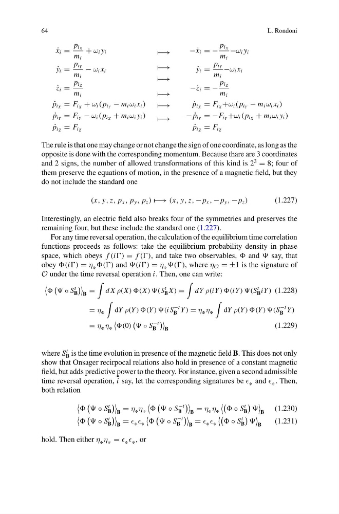
The rule is that one may change or not change the sign of one coordinate, as long as the
opposite is done with the corresponding momentum. Because thare are 3 coordinates
and 2 signs, the number of allowed transformations of this kind is 2
3
= 8; four of
them preserve the equations of motion, in the presence of a magnetic field, but they
do not include the standard one
(x, y, z, p x , p y , p z ) −→ (x, y, z, − p x , − p y , − p z )
(1.227)
Interestingly, an electric field also breaks four of the symmetries and preserves the
remaining four, but these include the standard one (1.227).
For any time reversal operation, the calculation of the equilibrium time correlation
functions proceeds as follows: take the equilibrium probability density in phase
space, which obeys f (i) = f ((), and take two observables, and say, that
obey (i) = η and (i) = η ((), where η O = ±1 is the signature of
O under the time reversal operation i. Then, one can write:
◦ S
t
B
B
=
d X ρ(X ) )(X ) )(S
t
B X ) =
dY ρ(iY ) )(iY ) )(S
t
B iY ) (1.228)
= η
dY ρ(Y ) )(Y ) )(i S
−t
B Y ) = η η
dY ρ(Y ) )(Y ) )(S
−t
B Y )
= η η
(0)
◦ S
−t
B
B
(1.229)
where S
t
B is the time evolution in presence of the magnetic field B. This does not only
show that Onsager recirpocal relations also hold in presence of a constant magnetic
field, but adds predictive power to the theory. For instance, given a second admissible
time reversal operation, ˜
i say, let the corresponding signatures be and . Then,
both relation
◦ S
t
B
B
= η η
◦ S
−t
B
B
= η η
◦ S
t
B
B
(1.230)
◦ S
t
B
B
=
◦ S
−t
B
B
=
◦ S
t
B
B
(1.231)
hold. Then either η η = , or
L. Rondoni
˙
x i =
p i X
m i
+ ω i y i
˙
y i =
p i Y
m i
− ω i x i
˙
z i =
p i Z
m i
˙
p i X = F i X + ω i ( p i Y − m i ω i x i )
˙
p i Y = F i Y − ω i ( p i X + m i ω i y i )
˙
p i Z = F i Z
−→
−→
−→
−→
−→
−→
− ˙
x i = −
p i X
m i
−ω i y i
˙
y i =
p i Y
m i
−ω i x i
−˙ z i = −
p i Z
m i
˙
p i X = F i X +ω i ( p i Y − m i ω i x i )
− ˙
p i Y = −F i Y +ω i ( p i X + m i ω i y i )
˙
p i Z = F i Z
The rule is that one may change or not change the sign of one coordinate, as long as the
opposite is done with the corresponding momentum. Because thare are 3 coordinates
and 2 signs, the number of allowed transformations of this kind is 2
3
= 8; four of
them preserve the equations of motion, in the presence of a magnetic field, but they
do not include the standard one
(x, y, z, p x , p y , p z ) −→ (x, y, z, − p x , − p y , − p z )
(1.227)
Interestingly, an electric field also breaks four of the symmetries and preserves the
remaining four, but these include the standard one (1.227).
For any time reversal operation, the calculation of the equilibrium time correlation
functions proceeds as follows: take the equilibrium probability density in phase
space, which obeys f (i) = f ((), and take two observables, and say, that
obey (i) = η and (i) = η ((), where η O = ±1 is the signature of
O under the time reversal operation i. Then, one can write:
◦ S
t
B
B
=
d X ρ(X ) )(X ) )(S
t
B X ) =
dY ρ(iY ) )(iY ) )(S
t
B iY ) (1.228)
= η
dY ρ(Y ) )(Y ) )(i S
−t
B Y ) = η η
dY ρ(Y ) )(Y ) )(S
−t
B Y )
= η η
(0)
◦ S
−t
B
B
(1.229)
where S
t
B is the time evolution in presence of the magnetic field B. This does not only
show that Onsager recirpocal relations also hold in presence of a constant magnetic
field, but adds predictive power to the theory. For instance, given a second admissible
time reversal operation, ˜
i say, let the corresponding signatures be and . Then,
both relation
◦ S
t
B
B
= η η
◦ S
−t
B
B
= η η
◦ S
t
B
B
(1.230)
◦ S
t
B
B
=
◦ S
−t
B
B
=
◦ S
t
B
B
(1.231)
hold. Then either η η = , or