

1 Introduction to Nonequilibrium Statistical Physics and Its Foundations
55
Fig. 1.14 Two snapshots of a billiard table with 11 balls. The notion of uniform mass distribution
begins to make sense; it improves if the balls are smaller and a larger number. In case the motion
is spontaneous and is subject to no friction, the direction of time is revealed by the transition from
ordered to disordered (uniform) mass distribution. This is achieved for practically whatever initial
impulse is given to a single ball. The reverse motion is not impossible, but exceedingly hard to
achieve (all balls should be extremely precisely aimed). Moreover, the ordered distribution would
turn into disorder, immediately after it has been created
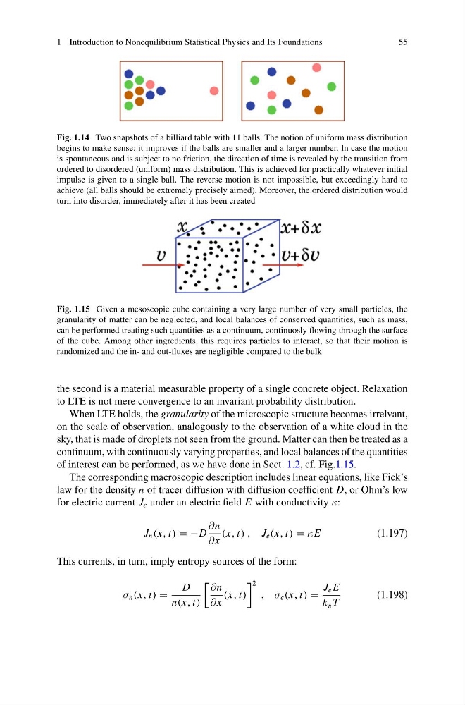
Fig. 1.15 Given a mesoscopic cube containing a very large number of very small particles, the
granularity of matter can be neglected, and local balances of conserved quantities, such as mass,
can be performed treating such quantities as a continuum, continuosly flowing through the surface
of the cube. Among other ingredients, this requires particles to interact, so that their motion is
randomized and the in- and out-fluxes are negligible compared to the bulk
the second is a material measurable property of a single concrete object. Relaxation
to LTE is not mere convergence to an invariant probability distribution.
When LTE holds, the granularity of the microscopic structure becomes irrelvant,
on the scale of observation, analogously to the observation of a white cloud in the
sky, that is made of droplets not seen from the ground. Matter can then be treated as a
continuum, with continuously varying properties, and local balances of the quantities
of interest can be performed, as we have done in Sect. 1.2, cf. Fig.1.15.
The corresponding macroscopic description includes linear equations, like Fick’s
law for the density n of tracer diffusion with diffusion coefficient D, or Ohm’s low
for electric current J e under an electric field E with conductivity κ:
J n (x, t) = −D
∂n
∂x
(x, t) , J e (x, t) = κE
(1.197)
This currents, in turn, imply entropy sources of the form:
σ n (x, t) =
D
n(x, t)
∂n
∂x
(x, t)
2
, σ e (x, t) =
J e E
k B T
(1.198)
55
Fig. 1.14 Two snapshots of a billiard table with 11 balls. The notion of uniform mass distribution
begins to make sense; it improves if the balls are smaller and a larger number. In case the motion
is spontaneous and is subject to no friction, the direction of time is revealed by the transition from
ordered to disordered (uniform) mass distribution. This is achieved for practically whatever initial
impulse is given to a single ball. The reverse motion is not impossible, but exceedingly hard to
achieve (all balls should be extremely precisely aimed). Moreover, the ordered distribution would
turn into disorder, immediately after it has been created
Fig. 1.15 Given a mesoscopic cube containing a very large number of very small particles, the
granularity of matter can be neglected, and local balances of conserved quantities, such as mass,
can be performed treating such quantities as a continuum, continuosly flowing through the surface
of the cube. Among other ingredients, this requires particles to interact, so that their motion is
randomized and the in- and out-fluxes are negligible compared to the bulk
the second is a material measurable property of a single concrete object. Relaxation
to LTE is not mere convergence to an invariant probability distribution.
When LTE holds, the granularity of the microscopic structure becomes irrelvant,
on the scale of observation, analogously to the observation of a white cloud in the
sky, that is made of droplets not seen from the ground. Matter can then be treated as a
continuum, with continuously varying properties, and local balances of the quantities
of interest can be performed, as we have done in Sect. 1.2, cf. Fig.1.15.
The corresponding macroscopic description includes linear equations, like Fick’s
law for the density n of tracer diffusion with diffusion coefficient D, or Ohm’s low
for electric current J e under an electric field E with conductivity κ:
J n (x, t) = −D
∂n
∂x
(x, t) , J e (x, t) = κE
(1.197)
This currents, in turn, imply entropy sources of the form:
σ n (x, t) =
D
n(x, t)
∂n
∂x
(x, t)
2
, σ e (x, t) =
J e E
k B T
(1.198)