

20
L. Rondoni
Introducing the following representation of δ function:
δ(x) =
1
2π
∞
−∞
dk e
ikx
(1.54)
we get:
P(z, t + τ |z
, t) =
1 +
+∞
n=1
1
n!
−
∂
∂z
n
M n (z, t, τ )
δ(z − z
)
(1.55)
which yields:
W (z, t + τ ) =
W (z , t)δ(z − z )dz −
∂
∂z
M 1 (z, t, τ )
W (z , t)δ(z − z )dz + · · ·
(1.56)
=
1 −
∂
∂z
M 1 +
1
2
∂ 2
∂z 2 M 2 + · · ·
W (z, t)
(1.57)
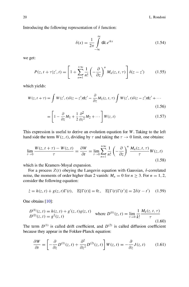
This expression is useful to derive an evolution equation for W . Taking to the left
hand side the term W (z, t), dividing by τ and taking the τ → 0 limit, one obtains:
lim
τ →0
W (z, t + τ ) − W (z, t)
τ
=
∂W
∂t
= lim
τ →0
+∞
n=1
1
n!
−
∂
∂z
n M n (z, t, τ )
τ
W (z, t)
(1.58)
which is the Kramers-Moyal expansion.
For a process Z (t) obeying the Langevin equation with Gaussian, δ-correlated
noise, the moments of order higher than 2 vanish: M n = 0 for n ≥ 3. For n = 1, 2,
consider the following equation:
˙
z = h(z, t) + g(z, t))(t), E[(t)] = 0;, E[(t))(t
)] = 2δ(t − t
) (1.59)
One obtains [10]:
D
(1)
(z, t) = h(z, t) + g
(z, t)g(z, t)
D
(2)
(z, t) = g
2
(z, t)
where D
(k)
(z, t) = lim
τ →0
1
k!
M k (z, t, τ )
τ
(1.60)
The term D
(1) is called drift coefficient, and D
(2) is called diffusion coefficient
because they appear in the Fokker-Planck equation:
∂W
∂t
=
−
∂
∂z
D
(1)
(z, t) +
∂
2
∂z 2 D
(2)
(z, t)
W (z, t) = −
∂
∂z
J (z, t)
(1.61)
L. Rondoni
Introducing the following representation of δ function:
δ(x) =
1
2π
∞
−∞
dk e
ikx
(1.54)
we get:
P(z, t + τ |z
, t) =
1 +
+∞
n=1
1
n!
−
∂
∂z
n
M n (z, t, τ )
δ(z − z
)
(1.55)
which yields:
W (z, t + τ ) =
W (z , t)δ(z − z )dz −
∂
∂z
M 1 (z, t, τ )
W (z , t)δ(z − z )dz + · · ·
(1.56)
=
1 −
∂
∂z
M 1 +
1
2
∂ 2
∂z 2 M 2 + · · ·
W (z, t)
(1.57)
This expression is useful to derive an evolution equation for W . Taking to the left
hand side the term W (z, t), dividing by τ and taking the τ → 0 limit, one obtains:
lim
τ →0
W (z, t + τ ) − W (z, t)
τ
=
∂W
∂t
= lim
τ →0
+∞
n=1
1
n!
−
∂
∂z
n M n (z, t, τ )
τ
W (z, t)
(1.58)
which is the Kramers-Moyal expansion.
For a process Z (t) obeying the Langevin equation with Gaussian, δ-correlated
noise, the moments of order higher than 2 vanish: M n = 0 for n ≥ 3. For n = 1, 2,
consider the following equation:
˙
z = h(z, t) + g(z, t))(t), E[(t)] = 0;, E[(t))(t
)] = 2δ(t − t
) (1.59)
One obtains [10]:
D
(1)
(z, t) = h(z, t) + g
(z, t)g(z, t)
D
(2)
(z, t) = g
2
(z, t)
where D
(k)
(z, t) = lim
τ →0
1
k!
M k (z, t, τ )
τ
(1.60)
The term D
(1) is called drift coefficient, and D
(2) is called diffusion coefficient
because they appear in the Fokker-Planck equation:
∂W
∂t
=
−
∂
∂z
D
(1)
(z, t) +
∂
2
∂z 2 D
(2)
(z, t)
W (z, t) = −
∂
∂z
J (z, t)
(1.61)