

5 Basics of Molecular Modeling and Molecular Simulation
211
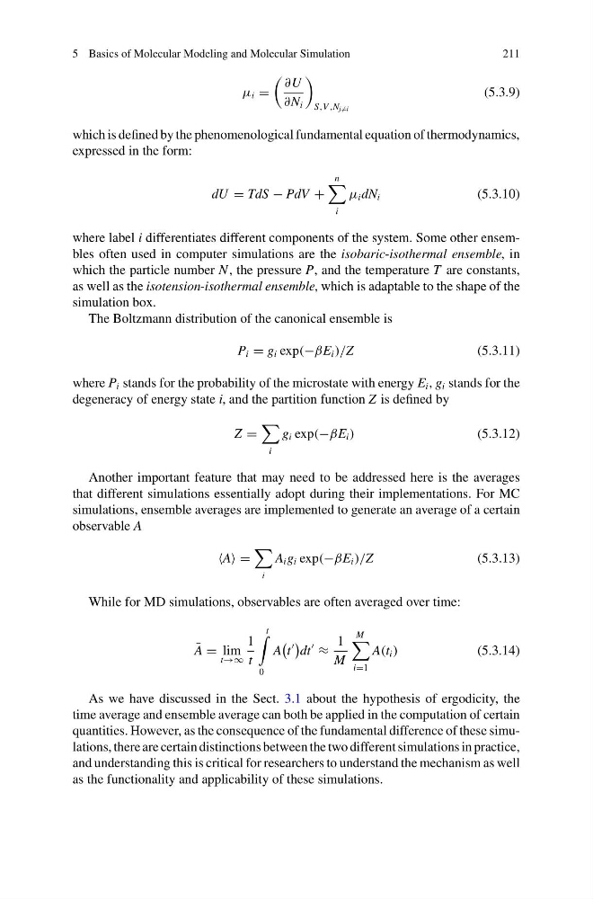
μ i =
∂U
∂N i
S,V ,N j =i
(5.3.9)
which is defined by the phenomenological fundamental equation of thermodynamics,
expressed in the form:
dU = TdS − PdV +
n
i
μ i dN i
(5.3.10)
where label i differentiates different components of the system. Some other ensembles often used in computer simulations are the isobaric-isothermal ensemble, in
which the particle number N , the pressure P, and the temperature T are constants,
as well as the isotension-isothermal ensemble, which is adaptable to the shape of the
simulation box.
The Boltzmann distribution of the canonical ensemble is
P i = g i exp(−βE i )/Z
(5.3.11)
where P i stands for the probability of the microstate with energy E i , g i stands for the
degeneracy of energy state i, and the partition function Z is defined by
Z =
i
g i exp(−βE i )
(5.3.12)
Another important feature that may need to be addressed here is the averages
that different simulations essentially adopt during their implementations. For MC
simulations, ensemble averages are implemented to generate an average of a certain
observable A
A =
i
A i g i exp(−βE i )/Z
(5.3.13)
While for MD simulations, observables are often averaged over time:
¯
A = lim
t→∞
1
t
t
0
A
t
dt
≈
1
M
M
i=1
A(t i )
(5.3.14)
As we have discussed in the Sect. 3.1 about the hypothesis of ergodicity, the
time average and ensemble average can both be applied in the computation of certain
quantities. However, as the consequence of the fundamental difference of these simulations, there are certain distinctions between the two different simulations in practice,
and understanding this is critical for researchers to understand the mechanism as well
as the functionality and applicability of these simulations.
211
μ i =
∂U
∂N i
S,V ,N j =i
(5.3.9)
which is defined by the phenomenological fundamental equation of thermodynamics,
expressed in the form:
dU = TdS − PdV +
n
i
μ i dN i
(5.3.10)
where label i differentiates different components of the system. Some other ensembles often used in computer simulations are the isobaric-isothermal ensemble, in
which the particle number N , the pressure P, and the temperature T are constants,
as well as the isotension-isothermal ensemble, which is adaptable to the shape of the
simulation box.
The Boltzmann distribution of the canonical ensemble is
P i = g i exp(−βE i )/Z
(5.3.11)
where P i stands for the probability of the microstate with energy E i , g i stands for the
degeneracy of energy state i, and the partition function Z is defined by
Z =
i
g i exp(−βE i )
(5.3.12)
Another important feature that may need to be addressed here is the averages
that different simulations essentially adopt during their implementations. For MC
simulations, ensemble averages are implemented to generate an average of a certain
observable A
A =
i
A i g i exp(−βE i )/Z
(5.3.13)
While for MD simulations, observables are often averaged over time:
¯
A = lim
t→∞
1
t
t
0
A
t
dt
≈
1
M
M
i=1
A(t i )
(5.3.14)
As we have discussed in the Sect. 3.1 about the hypothesis of ergodicity, the
time average and ensemble average can both be applied in the computation of certain
quantities. However, as the consequence of the fundamental difference of these simulations, there are certain distinctions between the two different simulations in practice,
and understanding this is critical for researchers to understand the mechanism as well
as the functionality and applicability of these simulations.