

202
C. Tang (唐晨宇) and Y. Wang (王延颋)
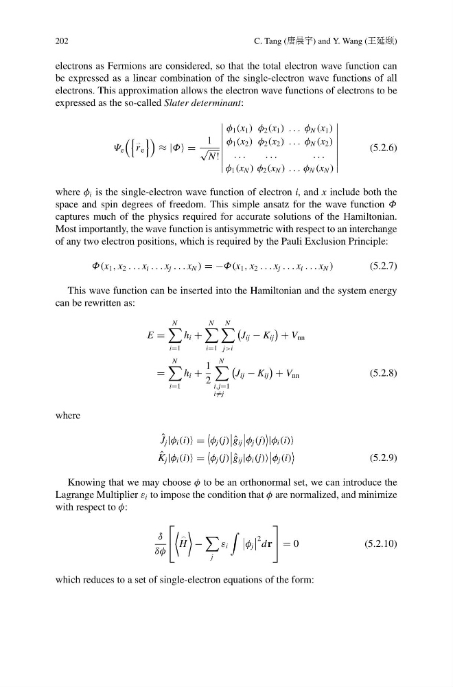
electrons as Fermions are considered, so that the total electron wave function can
be expressed as a linear combination of the single-electron wave functions of all
electrons. This approximation allows the electron wave functions of electrons to be
expressed as the so-called Slater determinant:
Ψ e
r e
≈ |Φ =
1
√
N !
φ 1 (x 1 ) φ 2 (x 1 ) . . . φ N (x 1 )
φ 1 (x 2 ) φ 2 (x 2 ) . . . φ N (x 2 )
. . .
. . .
. . .
φ 1 (x N ) φ 2 (x N ) . . . φ N (x N )
(5.2.6)
where φ i is the single-electron wave function of electron i, and x include both the
space and spin degrees of freedom. This simple ansatz for the wave function Φ
captures much of the physics required for accurate solutions of the Hamiltonian.
Most importantly, the wave function is antisymmetric with respect to an interchange
of any two electron positions, which is required by the Pauli Exclusion Principle:
Φ(x 1 , x 2 . . . x i . . . x j . . . x N ) = −Φ(x 1 , x 2 . . . x j . . . x i . . . x N )
(5.2.7)
This wave function can be inserted into the Hamiltonian and the system energy
can be rewritten as:
E =
N
i=1
h i +
N
i=1
N
j>i
J ij − K ij
+ V nn
=
N
i=1
h i +
1
2
N
i,j=1
i =j
J ij − K ij
+ V nn
(5.2.8)
where
ˆ
J j |φ i (i) =
φ j (j)
ˆ
g ij
φ j (j)
|φ i (i)
ˆ
K j |φ i (i) =
φ j (j)
ˆ
g ij |φ i (j)
φ j (i)
(5.2.9)
Knowing that we may choose φ to be an orthonormal set, we can introduce the
Lagrange Multiplier ε i to impose the condition that φ are normalized, and minimize
with respect to φ:
δ
δφ
⎡
⎣
H
−
j
ε i
φ j
2 d r
⎤
⎦ = 0
(5.2.10)
which reduces to a set of single-electron equations of the form:
C. Tang (唐晨宇) and Y. Wang (王延颋)
electrons as Fermions are considered, so that the total electron wave function can
be expressed as a linear combination of the single-electron wave functions of all
electrons. This approximation allows the electron wave functions of electrons to be
expressed as the so-called Slater determinant:
Ψ e
r e
≈ |Φ =
1
√
N !
φ 1 (x 1 ) φ 2 (x 1 ) . . . φ N (x 1 )
φ 1 (x 2 ) φ 2 (x 2 ) . . . φ N (x 2 )
. . .
. . .
. . .
φ 1 (x N ) φ 2 (x N ) . . . φ N (x N )
(5.2.6)
where φ i is the single-electron wave function of electron i, and x include both the
space and spin degrees of freedom. This simple ansatz for the wave function Φ
captures much of the physics required for accurate solutions of the Hamiltonian.
Most importantly, the wave function is antisymmetric with respect to an interchange
of any two electron positions, which is required by the Pauli Exclusion Principle:
Φ(x 1 , x 2 . . . x i . . . x j . . . x N ) = −Φ(x 1 , x 2 . . . x j . . . x i . . . x N )
(5.2.7)
This wave function can be inserted into the Hamiltonian and the system energy
can be rewritten as:
E =
N
i=1
h i +
N
i=1
N
j>i
J ij − K ij
+ V nn
=
N
i=1
h i +
1
2
N
i,j=1
i =j
J ij − K ij
+ V nn
(5.2.8)
where
ˆ
J j |φ i (i) =
φ j (j)
ˆ
g ij
φ j (j)
|φ i (i)
ˆ
K j |φ i (i) =
φ j (j)
ˆ
g ij |φ i (j)
φ j (i)
(5.2.9)
Knowing that we may choose φ to be an orthonormal set, we can introduce the
Lagrange Multiplier ε i to impose the condition that φ are normalized, and minimize
with respect to φ:
δ
δφ
⎡
⎣
H
−
j
ε i
φ j
2 d r
⎤
⎦ = 0
(5.2.10)
which reduces to a set of single-electron equations of the form: