

4 An Introduction to Emergence Dynamics in Complex Systems
187
By introducing z = x + iy, Eq. (4.139) is written as two real equations:
˙
x = K 1 (N +1/2)y
2
− K 1 x
2
/2 + K 2 (N − 1)xy − ωy + K 1 /2,
˙
y = −K 2 (N − 1/2)x
2
− K 2 y
2
/2 − K 1 (N + 1)xy + ωx + K 2 /2.
(4.140)
here K 1 = Kcosα, K 2 = Ksinα. The fixed points (x 1∼4 , y 1∼4 ) can be worked out by
setting ˙
x = 0, ˙
y = 0 as
x 1,2 =
(−ω ± A) sin α
K(2N cos 2α + 1)
,
(4.141a)
y 1,2 =
(−ω ± A) cos α
K(2N cos 2α + 1)
,
(4.141b)
x 3,4 =
sin α
K
+
[B ± N (B − 2 sin 2α)] cos α
K(N 2 + 2N cos 2α + 1)
,
(4.141c)
y 3,4 =
−ω(− cos α ± B sin α − K cos α)
K(N 2 + 2N cos 2α + 1)
.
(4.141d)
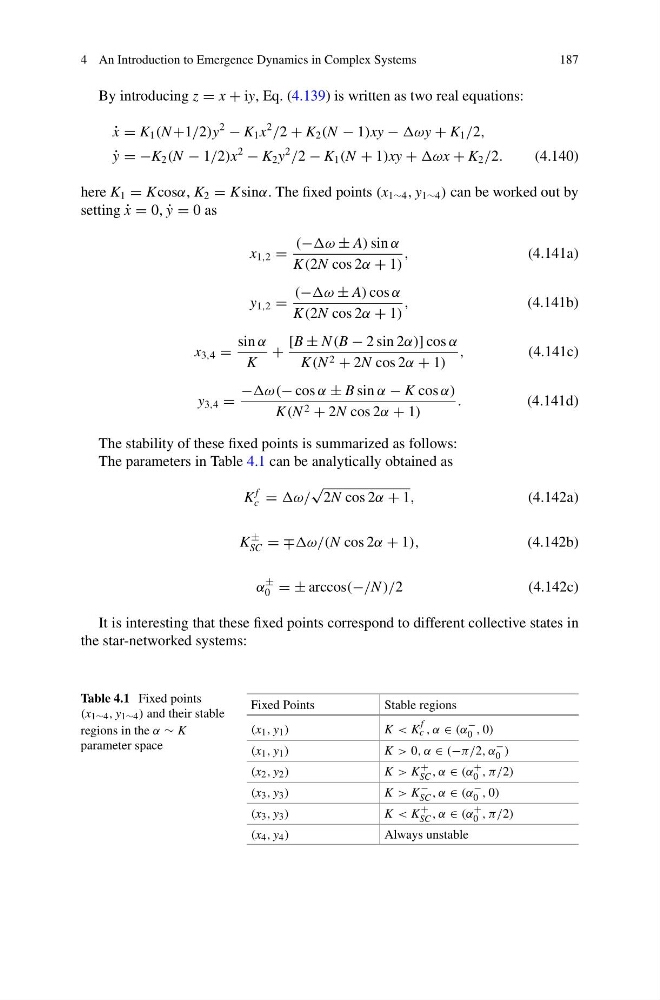
The stability of these fixed points is summarized as follows:
The parameters in Table 4.1 can be analytically obtained as
K
f
c = ω/
√
2N cos 2α + 1,
(4.142a)
K
±
SC = ∓ω/(N cos 2α + 1),
(4.142b)
α
±
0 = ± arccos(−/N )/2
(4.142c)
It is interesting that these fixed points correspond to different collective states in
the star-networked systems:
Table 4.1 Fixed points
(x 1∼4 , y 1∼4 ) and their stable
regions in the α ∼ K
parameter space
Fixed Points
Stable regions
(x 1 , y 1 )
K < K
f
c , α ∈ (α
−
0 , 0)
(x 1 , y 1 )
K > 0, α ∈ (−π/2, α
−
0 )
(x 2 , y 2 )
K > K
+
SC , α ∈ (α
+
0 , π/2)
(x 3 , y 3 )
K > K
−
SC , α ∈ (α
−
0 , 0)
(x 3 , y 3 )
K < K
+
SC , α ∈ (α
+
0 , π/2)
(x 4 , y 4 )
Always unstable
187
By introducing z = x + iy, Eq. (4.139) is written as two real equations:
˙
x = K 1 (N +1/2)y
2
− K 1 x
2
/2 + K 2 (N − 1)xy − ωy + K 1 /2,
˙
y = −K 2 (N − 1/2)x
2
− K 2 y
2
/2 − K 1 (N + 1)xy + ωx + K 2 /2.
(4.140)
here K 1 = Kcosα, K 2 = Ksinα. The fixed points (x 1∼4 , y 1∼4 ) can be worked out by
setting ˙
x = 0, ˙
y = 0 as
x 1,2 =
(−ω ± A) sin α
K(2N cos 2α + 1)
,
(4.141a)
y 1,2 =
(−ω ± A) cos α
K(2N cos 2α + 1)
,
(4.141b)
x 3,4 =
sin α
K
+
[B ± N (B − 2 sin 2α)] cos α
K(N 2 + 2N cos 2α + 1)
,
(4.141c)
y 3,4 =
−ω(− cos α ± B sin α − K cos α)
K(N 2 + 2N cos 2α + 1)
.
(4.141d)
The stability of these fixed points is summarized as follows:
The parameters in Table 4.1 can be analytically obtained as
K
f
c = ω/
√
2N cos 2α + 1,
(4.142a)
K
±
SC = ∓ω/(N cos 2α + 1),
(4.142b)
α
±
0 = ± arccos(−/N )/2
(4.142c)
It is interesting that these fixed points correspond to different collective states in
the star-networked systems:
Table 4.1 Fixed points
(x 1∼4 , y 1∼4 ) and their stable
regions in the α ∼ K
parameter space
Fixed Points
Stable regions
(x 1 , y 1 )
K < K
f
c , α ∈ (α
−
0 , 0)
(x 1 , y 1 )
K > 0, α ∈ (−π/2, α
−
0 )
(x 2 , y 2 )
K > K
+
SC , α ∈ (α
+
0 , π/2)
(x 3 , y 3 )
K > K
−
SC , α ∈ (α
−
0 , 0)
(x 3 , y 3 )
K < K
+
SC , α ∈ (α
+
0 , π/2)
(x 4 , y 4 )
Always unstable