

4 An Introduction to Emergence Dynamics in Complex Systems
139
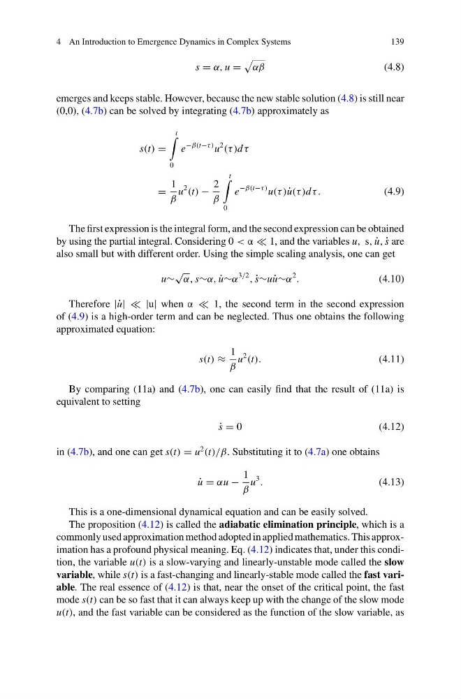
s = α, u =
αβ
(4.8)
emerges and keeps stable. However, because the new stable solution (4.8) is still near
(0,0), (4.7b) can be solved by integrating (4.7b) approximately as
s(t) =
t
0
e
−β(t−τ ) u
2
(τ )d τ
=
1
β
u
2
(t) −
2
β
t
0
e
−β(t−τ ) u(τ )˙ u(τ )d τ .
(4.9)
The first expression is the integral form, and the second expression can be obtained
by using the partial integral. Considering 0 < α 1, and the variables u, s, ˙
u, ˙
s are
also small but with different order. Using the simple scaling analysis, one can get
u∼
√ α, s∼α, ˙
u∼α
3/2
, ˙
s∼u ˙
u∼α
2
.
(4.10)
Therefore |˙ u| |u| when α 1, the second term in the second expression
of (4.9) is a high-order term and can be neglected. Thus one obtains the following
approximated equation:
s(t) ≈
1
β
u
2
(t).
(4.11)
By comparing (11a) and (4.7b), one can easily find that the result of (11a) is
equivalent to setting
˙
s = 0
(4.12)
in (4.7b), and one can get s(t) = u
2
(t)/β. Substituting it to (4.7a) one obtains
˙
u = αu −
1
β
u
3
.
(4.13)
This is a one-dimensional dynamical equation and can be easily solved.
The proposition (4.12) is called the adiabatic elimination principle, which is a
commonly used approximation method adopted in applied mathematics. This approximation has a profound physical meaning. Eq. (4.12) indicates that, under this condition, the variable u(t) is a slow-varying and linearly-unstable mode called the slow
variable, while s(t) is a fast-changing and linearly-stable mode called the fast variable. The real essence of (4.12) is that, near the onset of the critical point, the fast
mode s(t) can be so fast that it can always keep up with the change of the slow mode
u(t), and the fast variable can be considered as the function of the slow variable, as
139
s = α, u =
αβ
(4.8)
emerges and keeps stable. However, because the new stable solution (4.8) is still near
(0,0), (4.7b) can be solved by integrating (4.7b) approximately as
s(t) =
t
0
e
−β(t−τ ) u
2
(τ )d τ
=
1
β
u
2
(t) −
2
β
t
0
e
−β(t−τ ) u(τ )˙ u(τ )d τ .
(4.9)
The first expression is the integral form, and the second expression can be obtained
by using the partial integral. Considering 0 < α 1, and the variables u, s, ˙
u, ˙
s are
also small but with different order. Using the simple scaling analysis, one can get
u∼
√ α, s∼α, ˙
u∼α
3/2
, ˙
s∼u ˙
u∼α
2
.
(4.10)
Therefore |˙ u| |u| when α 1, the second term in the second expression
of (4.9) is a high-order term and can be neglected. Thus one obtains the following
approximated equation:
s(t) ≈
1
β
u
2
(t).
(4.11)
By comparing (11a) and (4.7b), one can easily find that the result of (11a) is
equivalent to setting
˙
s = 0
(4.12)
in (4.7b), and one can get s(t) = u
2
(t)/β. Substituting it to (4.7a) one obtains
˙
u = αu −
1
β
u
3
.
(4.13)
This is a one-dimensional dynamical equation and can be easily solved.
The proposition (4.12) is called the adiabatic elimination principle, which is a
commonly used approximation method adopted in applied mathematics. This approximation has a profound physical meaning. Eq. (4.12) indicates that, under this condition, the variable u(t) is a slow-varying and linearly-unstable mode called the slow
variable, while s(t) is a fast-changing and linearly-stable mode called the fast variable. The real essence of (4.12) is that, near the onset of the critical point, the fast
mode s(t) can be so fast that it can always keep up with the change of the slow mode
u(t), and the fast variable can be considered as the function of the slow variable, as