

126
Q. Wang
σ
v
j
= M ·
D
−∇μ
, σ
a
= 0, ∇ · σ
e
= −c∇μ, σ
s
= −pI + σ
v
, (3.119)
where
M =
2ηδ αk δ βl
0
λδ αk
,
(3.120)
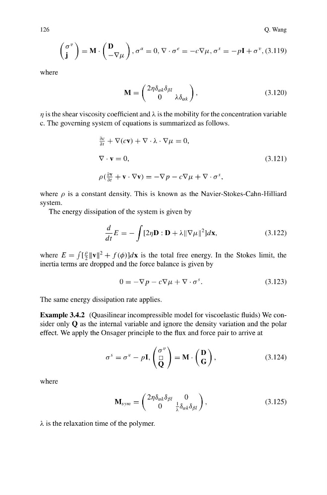
η is the shear viscosity coefficient and λ is the mobility for the concentration variable
c. The governing system of equations is summarized as follows.
∂c
∂t
+ ∇(cv) + ∇ · λ · ∇μ = 0,
∇ · v = 0,
ρ(
∂v
∂t
+ v · ∇v) = −∇ p − c∇μ + ∇ · σ
s
,
(3.121)
where ρ is a constant density. This is known as the Navier-Stokes-Cahn-Hilliard
system.
The energy dissipation of the system is given by
d
dt
E = −
[2ηD : D + λ∇μ
2
]dx,
(3.122)
where E =
[
ρ
2
v
2
+ f (φ)]dx is the total free energy. In the Stokes limit, the
inertia terms are dropped and the force balance is given by
0 = −∇ p − c∇μ + ∇ · σ
s
.
(3.123)
The same energy dissipation rate applies.
Example 3.4.2 (Quasilinear incompressible model for viscoelastic fluids) We consider only Q as the internal variable and ignore the density variation and the polar
effect. We apply the Onsager principle to the flux and force pair to arrive at
σ
s
= σ
v
− pI,
σ
v
Q
= M ·
D
G
,
(3.124)
where
M sym =
2ηδ αk δ βl
0
0
1
λ
δ αk δ βl
,
(3.125)
λ is the relaxation time of the polymer.
Q. Wang
σ
v
j
= M ·
D
−∇μ
, σ
a
= 0, ∇ · σ
e
= −c∇μ, σ
s
= −pI + σ
v
, (3.119)
where
M =
2ηδ αk δ βl
0
λδ αk
,
(3.120)
η is the shear viscosity coefficient and λ is the mobility for the concentration variable
c. The governing system of equations is summarized as follows.
∂c
∂t
+ ∇(cv) + ∇ · λ · ∇μ = 0,
∇ · v = 0,
ρ(
∂v
∂t
+ v · ∇v) = −∇ p − c∇μ + ∇ · σ
s
,
(3.121)
where ρ is a constant density. This is known as the Navier-Stokes-Cahn-Hilliard
system.
The energy dissipation of the system is given by
d
dt
E = −
[2ηD : D + λ∇μ
2
]dx,
(3.122)
where E =
[
ρ
2
v
2
+ f (φ)]dx is the total free energy. In the Stokes limit, the
inertia terms are dropped and the force balance is given by
0 = −∇ p − c∇μ + ∇ · σ
s
.
(3.123)
The same energy dissipation rate applies.
Example 3.4.2 (Quasilinear incompressible model for viscoelastic fluids) We consider only Q as the internal variable and ignore the density variation and the polar
effect. We apply the Onsager principle to the flux and force pair to arrive at
σ
s
= σ
v
− pI,
σ
v
Q
= M ·
D
G
,
(3.124)
where
M sym =
2ηδ αk δ βl
0
0
1
λ
δ αk δ βl
,
(3.125)
λ is the relaxation time of the polymer.