

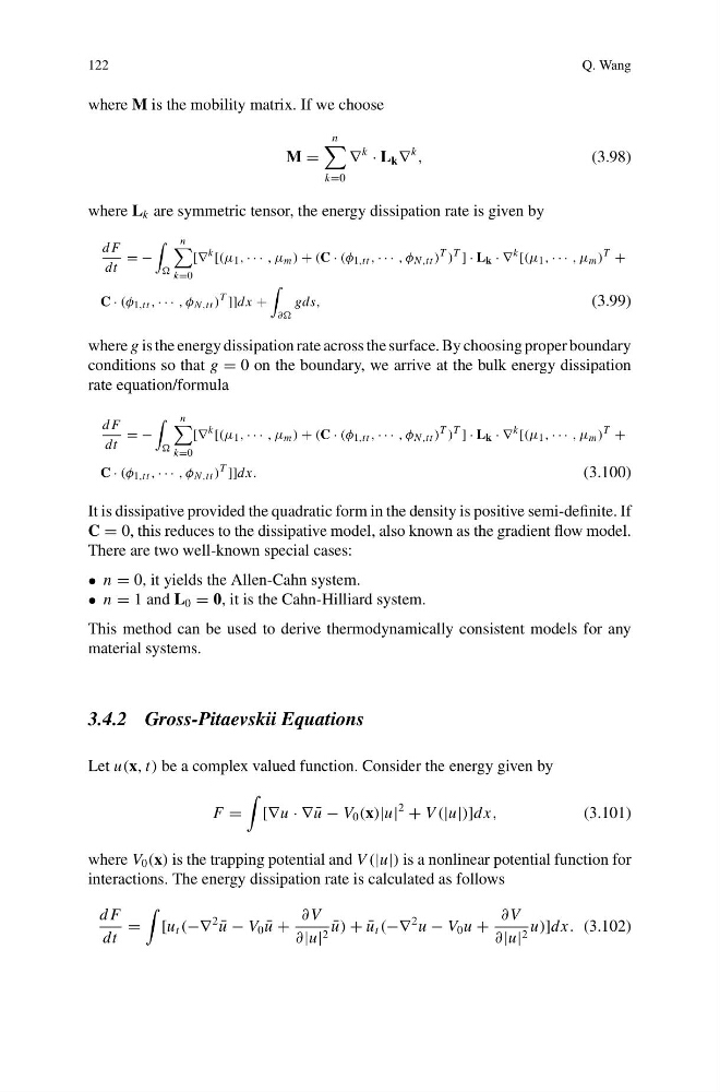
122
Q. Wang
where M is the mobility matrix. If we choose
M =
n
k=0
∇
k
· L k ∇
k
,
(3.98)
where L k are symmetric tensor, the energy dissipation rate is given by
d F
dt
= −
n
k=0
[∇
k [(μ 1 , · · · , μ m ) + (C · (φ 1,tt , · · · , φ N ,tt )
T )
T ] · L k · ∇
k [(μ 1 , · · · , μ m )
T +
C · (φ 1,tt , · · · , φ N ,tt )
T ]]dx +
∂∂
gds,
(3.99)
where g is the energy dissipation rate across the surface. By choosing proper boundary
conditions so that g = 0 on the boundary, we arrive at the bulk energy dissipation
rate equation/formula
d F
dt
= −
n
k=0
[∇
k [(μ 1 , · · · , μ m ) + (C · (φ 1,tt , · · · , φ N ,tt )
T )
T ] · L k · ∇
k [(μ 1 , · · · , μ m )
T +
C · (φ 1,tt , · · · , φ N ,tt )
T ]]dx.
(3.100)
It is dissipative provided the quadratic form in the density is positive semi-definite. If
C = 0, this reduces to the dissipative model, also known as the gradient flow model.
There are two well-known special cases:
• n = 0, it yields the Allen-Cahn system.
• n = 1 and L 0 = 0, it is the Cahn-Hilliard system.
This method can be used to derive thermodynamically consistent models for any
material systems.
3.4.2 Gross-Pitaevskii Equations
Let u(x, t) be a complex valued function. Consider the energy given by
F =
[∇u · ∇ ¯
u − V 0 (x)|u|
2
+ V (|u|)]dx,
(3.101)
where V 0 (x) is the trapping potential and V (|u|) is a nonlinear potential function for
interactions. The energy dissipation rate is calculated as follows
d F
dt
=
[u t (−∇
2
¯
u − V 0 ¯
u +
∂ V
∂|u| 2 ¯
u) + ¯
u t (−∇
2 u − V 0 u +
∂ V
∂|u| 2 u)]dx. (3.102)
Q. Wang
where M is the mobility matrix. If we choose
M =
n
k=0
∇
k
· L k ∇
k
,
(3.98)
where L k are symmetric tensor, the energy dissipation rate is given by
d F
dt
= −
n
k=0
[∇
k [(μ 1 , · · · , μ m ) + (C · (φ 1,tt , · · · , φ N ,tt )
T )
T ] · L k · ∇
k [(μ 1 , · · · , μ m )
T +
C · (φ 1,tt , · · · , φ N ,tt )
T ]]dx +
∂∂
gds,
(3.99)
where g is the energy dissipation rate across the surface. By choosing proper boundary
conditions so that g = 0 on the boundary, we arrive at the bulk energy dissipation
rate equation/formula
d F
dt
= −
n
k=0
[∇
k [(μ 1 , · · · , μ m ) + (C · (φ 1,tt , · · · , φ N ,tt )
T )
T ] · L k · ∇
k [(μ 1 , · · · , μ m )
T +
C · (φ 1,tt , · · · , φ N ,tt )
T ]]dx.
(3.100)
It is dissipative provided the quadratic form in the density is positive semi-definite. If
C = 0, this reduces to the dissipative model, also known as the gradient flow model.
There are two well-known special cases:
• n = 0, it yields the Allen-Cahn system.
• n = 1 and L 0 = 0, it is the Cahn-Hilliard system.
This method can be used to derive thermodynamically consistent models for any
material systems.
3.4.2 Gross-Pitaevskii Equations
Let u(x, t) be a complex valued function. Consider the energy given by
F =
[∇u · ∇ ¯
u − V 0 (x)|u|
2
+ V (|u|)]dx,
(3.101)
where V 0 (x) is the trapping potential and V (|u|) is a nonlinear potential function for
interactions. The energy dissipation rate is calculated as follows
d F
dt
=
[u t (−∇
2
¯
u − V 0 ¯
u +
∂ V
∂|u| 2 ¯
u) + ¯
u t (−∇
2 u − V 0 u +
∂ V
∂|u| 2 u)]dx. (3.102)