

2 On the Foundational Principles of Statistical Mechanics
97
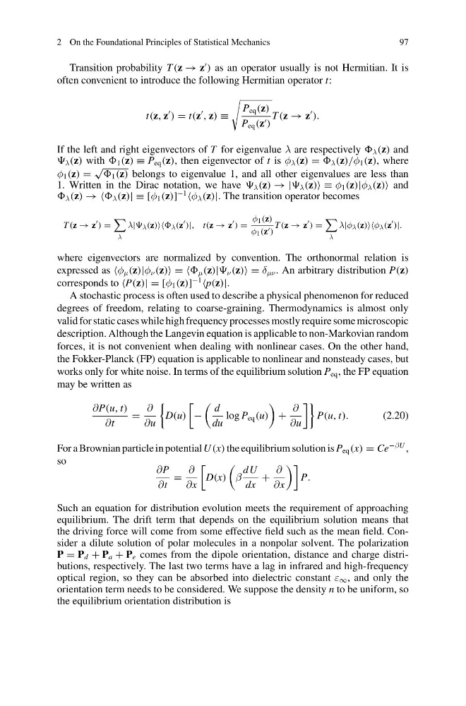
Transition probability T (z → z
) as an operator usually is not Hermitian. It is
often convenient to introduce the following Hermitian operator t:
t(z, z
) = t(z
, z) ≡
P eq (z)
P eq (z )
T (z → z
).
If the left and right eigenvectors of T for eigenvalue λ are respectively λ (z) and
λ (z) with 1 (z) ≡ P eq (z), then eigenvector of t is φ λ (z) = λ (z)/φ 1 (z), where
φ 1 (z) =
√ 1 (z) belongs to eigenvalue 1, and all other eigenvalues are less than
1. Written in the Dirac notation, we have λ (z) → | λ (z) ≡ φ 1 (z)|φ λ (z) and
λ (z) → → λ (z)| ≡ [φ 1 (z)]
−1
φ λ (z)|. The transition operator becomes
T (z → z
) =
λ
λ| λ (z) λ (z
)|, t(z → z
) =
φ 1 (z)
φ 1 (z )
T (z → z
) =
λ
λ|φ λ (z)φ λ (z
)|.
where eigenvectors are normalized by convention. The orthonormal relation is
expressed as φ μ (z)|φ ν (z) = = μ (z)| ν (z) = δ μν . An arbitrary distribution P(z)
corresponds to P(z)| = [φ 1 (z)]
−1
p(z)|.
A stochastic process is often used to describe a physical phenomenon for reduced
degrees of freedom, relating to coarse-graining. Thermodynamics is almost only
valid for static cases while high frequency processes mostly require some microscopic
description. Although the Langevin equation is applicable to non-Markovian random
forces, it is not convenient when dealing with nonlinear cases. On the other hand,
the Fokker-Planck (FP) equation is applicable to nonlinear and nonsteady cases, but
works only for white noise. In terms of the equilibrium solution P eq , the FP equation
may be written as
∂P(u, t)
∂t
=
∂
∂u
D(u)
−
d
du
log P eq (u)
+
∂
∂u
P(u, t).
(2.20)
For a Brownian particle in potential U (x) the equilibrium solution is P eq (x) = Ce
−βU ,
so
∂P
∂t
=
∂
∂x
D(x)
β
dU
dx
+
∂
∂x
P.
Such an equation for distribution evolution meets the requirement of approaching
equilibrium. The drift term that depends on the equilibrium solution means that
the driving force will come from some effective field such as the mean field. Consider a dilute solution of polar molecules in a nonpolar solvent. The polarization
P = P d + P a + P e comes from the dipole orientation, distance and charge distributions, respectively. The last two terms have a lag in infrared and high-frequency
optical region, so they can be absorbed into dielectric constant ε ∞ , and only the
orientation term needs to be considered. We suppose the density n to be uniform, so
the equilibrium orientation distribution is
97
Transition probability T (z → z
) as an operator usually is not Hermitian. It is
often convenient to introduce the following Hermitian operator t:
t(z, z
) = t(z
, z) ≡
P eq (z)
P eq (z )
T (z → z
).
If the left and right eigenvectors of T for eigenvalue λ are respectively λ (z) and
λ (z) with 1 (z) ≡ P eq (z), then eigenvector of t is φ λ (z) = λ (z)/φ 1 (z), where
φ 1 (z) =
√ 1 (z) belongs to eigenvalue 1, and all other eigenvalues are less than
1. Written in the Dirac notation, we have λ (z) → | λ (z) ≡ φ 1 (z)|φ λ (z) and
λ (z) → → λ (z)| ≡ [φ 1 (z)]
−1
φ λ (z)|. The transition operator becomes
T (z → z
) =
λ
λ| λ (z) λ (z
)|, t(z → z
) =
φ 1 (z)
φ 1 (z )
T (z → z
) =
λ
λ|φ λ (z)φ λ (z
)|.
where eigenvectors are normalized by convention. The orthonormal relation is
expressed as φ μ (z)|φ ν (z) = = μ (z)| ν (z) = δ μν . An arbitrary distribution P(z)
corresponds to P(z)| = [φ 1 (z)]
−1
p(z)|.
A stochastic process is often used to describe a physical phenomenon for reduced
degrees of freedom, relating to coarse-graining. Thermodynamics is almost only
valid for static cases while high frequency processes mostly require some microscopic
description. Although the Langevin equation is applicable to non-Markovian random
forces, it is not convenient when dealing with nonlinear cases. On the other hand,
the Fokker-Planck (FP) equation is applicable to nonlinear and nonsteady cases, but
works only for white noise. In terms of the equilibrium solution P eq , the FP equation
may be written as
∂P(u, t)
∂t
=
∂
∂u
D(u)
−
d
du
log P eq (u)
+
∂
∂u
P(u, t).
(2.20)
For a Brownian particle in potential U (x) the equilibrium solution is P eq (x) = Ce
−βU ,
so
∂P
∂t
=
∂
∂x
D(x)
β
dU
dx
+
∂
∂x
P.
Such an equation for distribution evolution meets the requirement of approaching
equilibrium. The drift term that depends on the equilibrium solution means that
the driving force will come from some effective field such as the mean field. Consider a dilute solution of polar molecules in a nonpolar solvent. The polarization
P = P d + P a + P e comes from the dipole orientation, distance and charge distributions, respectively. The last two terms have a lag in infrared and high-frequency
optical region, so they can be absorbed into dielectric constant ε ∞ , and only the
orientation term needs to be considered. We suppose the density n to be uniform, so
the equilibrium orientation distribution is