

328
6 Shocks and Surprises: Refining the Elementary Model
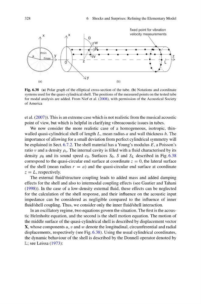
Fig. 6.38 (a) Polar graph of the elliptical cross-section of the tube. (b) Notations and coordinate
systems used for the quasi-cylindrical shell. The positions of the measured points on the tested tube
for modal analysis are added. From Nief et al. (2008), with permission of the Acoustical Society
of America
et al. (2007)). This is an extreme case which is not realistic from the musical acoustic
point of view, but which is helpful in clarifying vibroacoustic issues in tubes.
We now consider the more realistic case of a homogeneous, isotropic, thinwalled quasi-cylindrical shell of length L, mean radius a and wall thickness h. The
importance of allowing for a small deviation from perfect cylindrical symmetry will
be explained in Sect. 6.7.2. The shell material has a Young’s modulus E, a Poisson’s
ratio ν and a density ρ s . The internal cavity is filled with a fluid characterised by its
density ρ 0 and its sound speed c 0 . Surfaces S 0 , S and S L described in Fig. 6.38
correspond to the quasi-circular end surface at coordinate z = 0, the lateral surface
of the shell (mean radius r = a) and the quasi-circular end surface at coordinate
z = L, respectively.
The external fluid/structure coupling leads to added mass and added damping
effects for the shell and also to intermodal coupling effects (see Gautier and Tahani
(1998)). In the case of a low-density external fluid, these effects can be neglected
for the calculation of the shell response, and their influence on the acoustic input
impedance can be considered as negligible compared to the influence of inner
fluid/shell coupling. Thus, we consider only the inner fluid/shell interaction.
In an oscillatory regime, two equations govern the situation. The first is the acoustic Helmholtz equation, and the second is the shell motion equation. The motion of
the middle surface of the quasi-cylindrical shell is described by displacement vector
X, whose components u, v and w denote the longitudinal, circumferential and radial
displacements, respectively (see Fig. 6.38). Using the usual cylindrical coordinates,
the dynamic behaviour of the shell is described by the Donnell operator denoted by
L; see Leissa (1973):
6 Shocks and Surprises: Refining the Elementary Model
Fig. 6.38 (a) Polar graph of the elliptical cross-section of the tube. (b) Notations and coordinate
systems used for the quasi-cylindrical shell. The positions of the measured points on the tested tube
for modal analysis are added. From Nief et al. (2008), with permission of the Acoustical Society
of America
et al. (2007)). This is an extreme case which is not realistic from the musical acoustic
point of view, but which is helpful in clarifying vibroacoustic issues in tubes.
We now consider the more realistic case of a homogeneous, isotropic, thinwalled quasi-cylindrical shell of length L, mean radius a and wall thickness h. The
importance of allowing for a small deviation from perfect cylindrical symmetry will
be explained in Sect. 6.7.2. The shell material has a Young’s modulus E, a Poisson’s
ratio ν and a density ρ s . The internal cavity is filled with a fluid characterised by its
density ρ 0 and its sound speed c 0 . Surfaces S 0 , S and S L described in Fig. 6.38
correspond to the quasi-circular end surface at coordinate z = 0, the lateral surface
of the shell (mean radius r = a) and the quasi-circular end surface at coordinate
z = L, respectively.
The external fluid/structure coupling leads to added mass and added damping
effects for the shell and also to intermodal coupling effects (see Gautier and Tahani
(1998)). In the case of a low-density external fluid, these effects can be neglected
for the calculation of the shell response, and their influence on the acoustic input
impedance can be considered as negligible compared to the influence of inner
fluid/shell coupling. Thus, we consider only the inner fluid/shell interaction.
In an oscillatory regime, two equations govern the situation. The first is the acoustic Helmholtz equation, and the second is the shell motion equation. The motion of
the middle surface of the quasi-cylindrical shell is described by displacement vector
X, whose components u, v and w denote the longitudinal, circumferential and radial
displacements, respectively (see Fig. 6.38). Using the usual cylindrical coordinates,
the dynamic behaviour of the shell is described by the Donnell operator denoted by
L; see Leissa (1973):