

4.3 Bore Profiles of Brass Instruments
131
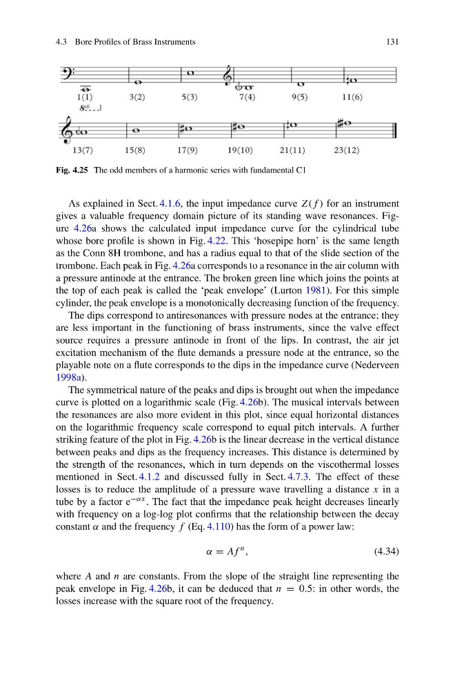
Fig. 4.25 The odd members of a harmonic series with fundamental C1
As explained in Sect. 4.1.6, the input impedance curve Z(f ) for an instrument
gives a valuable frequency domain picture of its standing wave resonances. Figure 4.26a shows the calculated input impedance curve for the cylindrical tube
whose bore profile is shown in Fig. 4.22. This ‘hosepipe horn’ is the same length
as the Conn 8H trombone, and has a radius equal to that of the slide section of the
trombone. Each peak in Fig. 4.26a corresponds to a resonance in the air column with
a pressure antinode at the entrance. The broken green line which joins the points at
the top of each peak is called the ‘peak envelope’ (Lurton 1981). For this simple
cylinder, the peak envelope is a monotonically decreasing function of the frequency.
The dips correspond to antiresonances with pressure nodes at the entrance; they
are less important in the functioning of brass instruments, since the valve effect
source requires a pressure antinode in front of the lips. In contrast, the air jet
excitation mechanism of the flute demands a pressure node at the entrance, so the
playable note on a flute corresponds to the dips in the impedance curve (Nederveen
1998a).
The symmetrical nature of the peaks and dips is brought out when the impedance
curve is plotted on a logarithmic scale (Fig. 4.26b). The musical intervals between
the resonances are also more evident in this plot, since equal horizontal distances
on the logarithmic frequency scale correspond to equal pitch intervals. A further
striking feature of the plot in Fig. 4.26b is the linear decrease in the vertical distance
between peaks and dips as the frequency increases. This distance is determined by
the strength of the resonances, which in turn depends on the viscothermal losses
mentioned in Sect. 4.1.2 and discussed fully in Sect. 4.7.3. The effect of these
losses is to reduce the amplitude of a pressure wave travelling a distance x in a
tube by a factor e −αx . The fact that the impedance peak height decreases linearly
with frequency on a log-log plot confirms that the relationship between the decay
constant α and the frequency f (Eq. 4.110) has the form of a power law:
α = Af
n ,
(4.34)
where A and n are constants. From the slope of the straight line representing the
peak envelope in Fig. 4.26b, it can be deduced that n = 0.5: in other words, the
losses increase with the square root of the frequency.
131
Fig. 4.25 The odd members of a harmonic series with fundamental C1
As explained in Sect. 4.1.6, the input impedance curve Z(f ) for an instrument
gives a valuable frequency domain picture of its standing wave resonances. Figure 4.26a shows the calculated input impedance curve for the cylindrical tube
whose bore profile is shown in Fig. 4.22. This ‘hosepipe horn’ is the same length
as the Conn 8H trombone, and has a radius equal to that of the slide section of the
trombone. Each peak in Fig. 4.26a corresponds to a resonance in the air column with
a pressure antinode at the entrance. The broken green line which joins the points at
the top of each peak is called the ‘peak envelope’ (Lurton 1981). For this simple
cylinder, the peak envelope is a monotonically decreasing function of the frequency.
The dips correspond to antiresonances with pressure nodes at the entrance; they
are less important in the functioning of brass instruments, since the valve effect
source requires a pressure antinode in front of the lips. In contrast, the air jet
excitation mechanism of the flute demands a pressure node at the entrance, so the
playable note on a flute corresponds to the dips in the impedance curve (Nederveen
1998a).
The symmetrical nature of the peaks and dips is brought out when the impedance
curve is plotted on a logarithmic scale (Fig. 4.26b). The musical intervals between
the resonances are also more evident in this plot, since equal horizontal distances
on the logarithmic frequency scale correspond to equal pitch intervals. A further
striking feature of the plot in Fig. 4.26b is the linear decrease in the vertical distance
between peaks and dips as the frequency increases. This distance is determined by
the strength of the resonances, which in turn depends on the viscothermal losses
mentioned in Sect. 4.1.2 and discussed fully in Sect. 4.7.3. The effect of these
losses is to reduce the amplitude of a pressure wave travelling a distance x in a
tube by a factor e −αx . The fact that the impedance peak height decreases linearly
with frequency on a log-log plot confirms that the relationship between the decay
constant α and the frequency f (Eq. 4.110) has the form of a power law:
α = Af
n ,
(4.34)
where A and n are constants. From the slope of the straight line representing the
peak envelope in Fig. 4.26b, it can be deduced that n = 0.5: in other words, the
losses increase with the square root of the frequency.