

5 Phase-Field-Crystal Model: A Tool for Probing Atoms in TSV
113
(a)
(b)
(c)
(d)
(e)
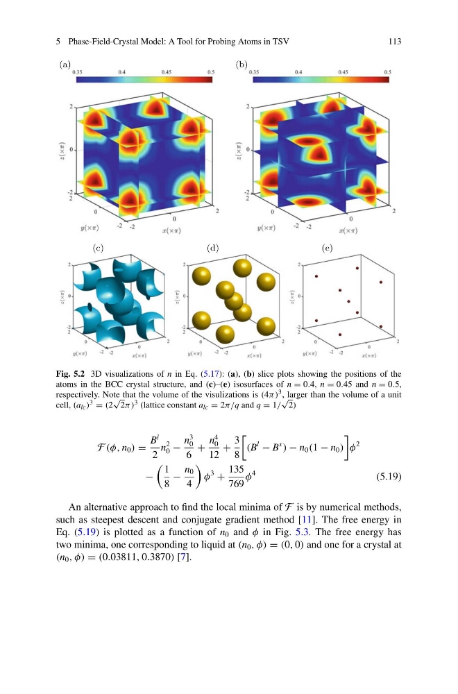
Fig. 5.2 3D visualizations of n in Eq. (5.17): (a), (b) slice plots showing the positions of the
atoms in the BCC crystal structure, and (c)–(e) isosurfaces of n = 0.4, n = 0.45 and n = 0.5,
respectively. Note that the volume of the visulizations is (4π) 3 , larger than the volume of a unit
cell, (a lc ) 3 = (2
√
2π) 3 (lattice constant a lc = 2π/q and q = 1/
√
2)
F (φ, n 0 ) =
B
l
2
n
2
0 −
n
3
0
6
+
n
4
0
12
+
3
8
(B
l
− B
x
) − n 0 (1 − n 0 )
φ
2
−
1
8
−
n 0
4
φ
3
+
135
769
φ
4
(5.19)
An alternative approach to find the local minima of F is by numerical methods,
such as steepest descent and conjugate gradient method [11]. The free energy in
Eq. (5.19) is plotted as a function of n 0 and φ in Fig. 5.3. The free energy has
two minima, one corresponding to liquid at (n 0 , φ) = (0, 0) and one for a crystal at
(n 0 , φ) = (0.03811, 0.3870) [7].
113
(a)
(b)
(c)
(d)
(e)
Fig. 5.2 3D visualizations of n in Eq. (5.17): (a), (b) slice plots showing the positions of the
atoms in the BCC crystal structure, and (c)–(e) isosurfaces of n = 0.4, n = 0.45 and n = 0.5,
respectively. Note that the volume of the visulizations is (4π) 3 , larger than the volume of a unit
cell, (a lc ) 3 = (2
√
2π) 3 (lattice constant a lc = 2π/q and q = 1/
√
2)
F (φ, n 0 ) =
B
l
2
n
2
0 −
n
3
0
6
+
n
4
0
12
+
3
8
(B
l
− B
x
) − n 0 (1 − n 0 )
φ
2
−
1
8
−
n 0
4
φ
3
+
135
769
φ
4
(5.19)
An alternative approach to find the local minima of F is by numerical methods,
such as steepest descent and conjugate gradient method [11]. The free energy in
Eq. (5.19) is plotted as a function of n 0 and φ in Fig. 5.3. The free energy has
two minima, one corresponding to liquid at (n 0 , φ) = (0, 0) and one for a crystal at
(n 0 , φ) = (0.03811, 0.3870) [7].