

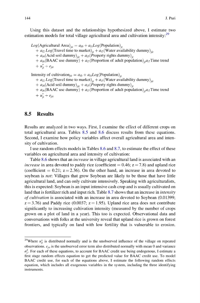
Using this dataset and the relationships hypothesized above, I estimate two
estimation models for total village agricultural area and cultivation intensity:
29
Log Agricultural Area
ð
Þ jit ¼ a i0 þ a i1 Log Population
ð
Þ jt
þ a i2 Log Travel time to market
ð
Þ jt þ a i3 Water availability dummy
ð
Þ jit
þ a i4 Acid soil dummy
ð
Þ jit þ a i5 Property rights dummy
ð
Þ jt
þ a i6 BAAC use dummy
ð
Þ þ a i7 Proportion of adult population
ð
Þ jt a i7 Time trend
þ u
*
ji þ ε jit
Intensity of cultivation jit ¼ a i0 þ a i1 Log Population
ð
Þ jt
þ a i2 Log Travel time to market
ð
Þ jt þ a i3 Water availability dummy
ð
Þ jit
þ a i4 Acid soil dummy
ð
Þ jit þ a i5 Property rights dummy
ð
Þ jt
þ a i6 BAAC use dummy
ð
Þ þ a i7 Proportion of adult population
ð
Þ jt a i7 Time trend
þ u
*
ji þ ε jit
8.5 Results
Results are analyzed in two ways. First, I examine the effect of different crops on
total agricultural area. Tables 8.5 and 8.6 discuss results from these equations.
Second, I examine how policy variables affect overall agricultural area and intensity of cultivation.
I use random effects models in Tables 8.6 and 8.7, to estimate the effect of these
variables on agricultural area and intensity of cultivation:
Table 8.6 shows that an increase in village agricultural land is associated with an
increase in area devoted to paddy rice (coefficient ¼ 0.46; z ¼ 7.8) and upland rice
(coefficient ¼ 0.21; z ¼ 2.36). On the other hand, an increase in area devoted to
soybean is not: Villages that grow Soybean are likely to be those that have little
agricultural land, and can only cultivate intensively. Speaking with agriculturalists,
this is expected: Soybean is an input intensive cash crop and is usually cultivated on
land that is fertilizer rich and input rich. Table 8.7 shows that an increase in intensity
of cultivation is associated with an increase in area devoted to Soybean (0.01399;
z ¼ 3.76) and Paddy rice (0.0037; z ¼ 1.95). Upland rice area does not contribute
significantly to increasing cultivation intensity (measured by the number of crops
grown on a plot of land in a year). This too is expected. Observational data and
conversations with folks at the university reveal that upland rice is grown on forest
frontiers, and typically on land with low fertility that is vulnerable to erosion.
29 Where u
Ã
ji is distributed normally and is the unobserved influence of the village on repeated
observations. ε jit is the unobserved error term also distributed normally with mean 0 and variance
σ
2
ε . For each of these equations, to account for BAAC credit use being endogenous, I estimate a
first stage random effects equation to get the predicted value for BAAC credit use. To model
BAAC credit use, for each of the equations above, I estimate the following random effects
equation, which includes all exogenous variables in the system, including the three identifying
instruments.
144
J. Puri
estimation models for total village agricultural area and cultivation intensity:
29
Log Agricultural Area
ð
Þ jit ¼ a i0 þ a i1 Log Population
ð
Þ jt
þ a i2 Log Travel time to market
ð
Þ jt þ a i3 Water availability dummy
ð
Þ jit
þ a i4 Acid soil dummy
ð
Þ jit þ a i5 Property rights dummy
ð
Þ jt
þ a i6 BAAC use dummy
ð
Þ þ a i7 Proportion of adult population
ð
Þ jt a i7 Time trend
þ u
*
ji þ ε jit
Intensity of cultivation jit ¼ a i0 þ a i1 Log Population
ð
Þ jt
þ a i2 Log Travel time to market
ð
Þ jt þ a i3 Water availability dummy
ð
Þ jit
þ a i4 Acid soil dummy
ð
Þ jit þ a i5 Property rights dummy
ð
Þ jt
þ a i6 BAAC use dummy
ð
Þ þ a i7 Proportion of adult population
ð
Þ jt a i7 Time trend
þ u
*
ji þ ε jit
8.5 Results
Results are analyzed in two ways. First, I examine the effect of different crops on
total agricultural area. Tables 8.5 and 8.6 discuss results from these equations.
Second, I examine how policy variables affect overall agricultural area and intensity of cultivation.
I use random effects models in Tables 8.6 and 8.7, to estimate the effect of these
variables on agricultural area and intensity of cultivation:
Table 8.6 shows that an increase in village agricultural land is associated with an
increase in area devoted to paddy rice (coefficient ¼ 0.46; z ¼ 7.8) and upland rice
(coefficient ¼ 0.21; z ¼ 2.36). On the other hand, an increase in area devoted to
soybean is not: Villages that grow Soybean are likely to be those that have little
agricultural land, and can only cultivate intensively. Speaking with agriculturalists,
this is expected: Soybean is an input intensive cash crop and is usually cultivated on
land that is fertilizer rich and input rich. Table 8.7 shows that an increase in intensity
of cultivation is associated with an increase in area devoted to Soybean (0.01399;
z ¼ 3.76) and Paddy rice (0.0037; z ¼ 1.95). Upland rice area does not contribute
significantly to increasing cultivation intensity (measured by the number of crops
grown on a plot of land in a year). This too is expected. Observational data and
conversations with folks at the university reveal that upland rice is grown on forest
frontiers, and typically on land with low fertility that is vulnerable to erosion.
29 Where u
Ã
ji is distributed normally and is the unobserved influence of the village on repeated
observations. ε jit is the unobserved error term also distributed normally with mean 0 and variance
σ
2
ε . For each of these equations, to account for BAAC credit use being endogenous, I estimate a
first stage random effects equation to get the predicted value for BAAC credit use. To model
BAAC credit use, for each of the equations above, I estimate the following random effects
equation, which includes all exogenous variables in the system, including the three identifying
instruments.
144
J. Puri