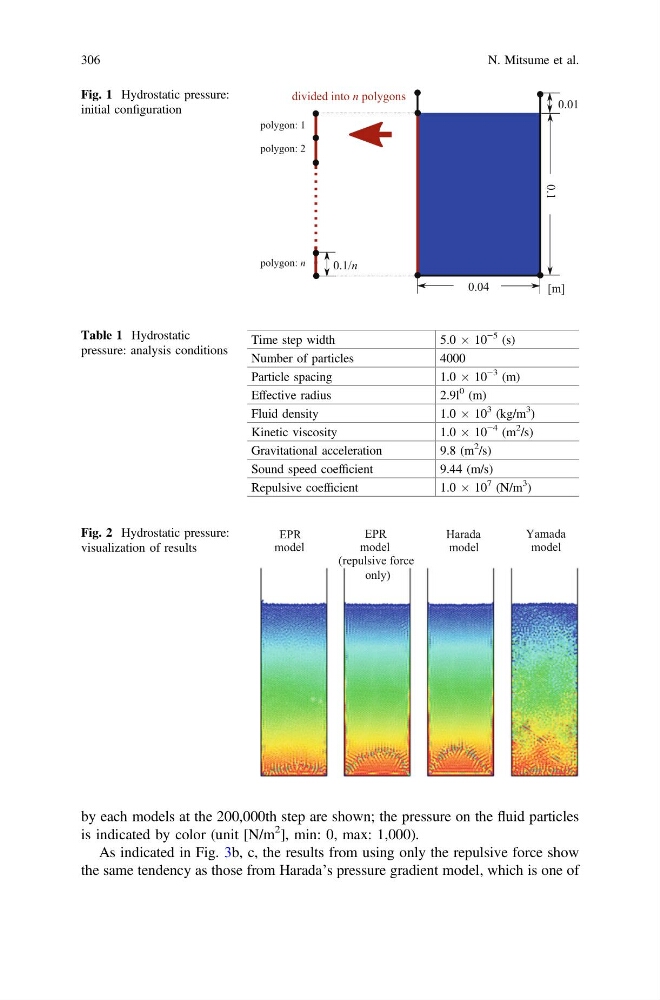
by each models at the 200,000th step are shown; the pressure on the fluid particles
is indicated by color (unit [N/m
2 ], min: 0, max: 1,000).
As indicated in Fig. 3b, c, the results from using only the repulsive force show
the same tendency as those from Harada’s pressure gradient model, which is one of
0.04
0.1
[m]
polygon: 1
polygon: 2
polygon: n
0.1/n
divided into n polygons
0.01
Fig. 1 Hydrostatic pressure:
initial configuration
Table 1 Hydrostatic
pressure: analysis conditions
Time step width
5.0 Â 10
−5 (s)
Number of particles
4000
Particle spacing
1.0 Â 10
−3 (m)
Effective radius
2.9l
0 (m)
Fluid density
1.0 Â 10
3 (kg/m
3
)
Kinetic viscosity
1.0 Â 10
−4 (m
2
/s)
Gravitational acceleration
9.8 (m
2
/s)
Sound speed coefficient
9.44 (m/s)
Repulsive coefficient
1.0 Â 10
7 (N/m
3
)
Harada
model
Yamada
model
EPR
model
EPR
model
(repulsive force
only)
Fig. 2 Hydrostatic pressure:
visualization of results
306
N. Mitsume et al.