

Endogenous variables:
V y K y ; i y
À
Á
expected total system cost ($)
C y K y ; i; dK y
À
Á
yearly system cost incurred in year y ($/year)
K y
capacity mix of power plants and power storage facilities (GW)
Kp y;p
capacity of p-th type of power plant in year y (GW)
dKp y;p
newly constructed capacity of p-th type of power plant in year
y (GW)
X p;t;d;y
output of p-th type of power plant in day d at time t and year
y (GW)
Ks1 y;s
kW capacity of s-th type of power storage facility in year y (GW)
Ks2 y;s
kWh capacity of s-th type of power storage facility in year y (GWh)
dKs1 y;s
newly constructed kW capacity of s-th type of power storage
facility in year y (GW)
dKs2 y;s
newly constructed kWh capacity of s-th type of power storage
facility in year y (GWh)
Cha s;d;t;y
input of s-th type of power storage facility in day d at time t and
year y (GW)
Dis s;d;t;y
output of s-th type of power storage facility in day d at time t and
year y (GW)
Ss s;d;t;y
stored energy of s-th type of power storage facility in day d at time
t and year y (GWh)
Save d;t;y
electricity demand saving in day d at time t and year y (GWh).
where p 2 {1: Nuclear, 2: Coal, 3: LNG CC, 4: LNG ST, 5: Oil, 6: Hydro}, s 2 {1:
Pumped hydro, 2: NAS battery}, d 2 {1, 2, …, 4}, t 2 {1, 2, …, 24}, y 2 {0, 1, …,
18}, i y : state of nuclear power plants availability in year y (i y = {0: nuclear power
unavailable, 1: nuclear available}).
2.1.1 Objective Function
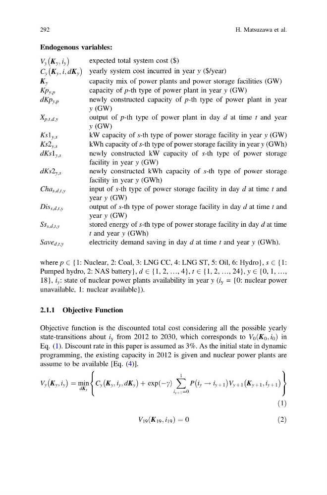
Objective function is the discounted total cost considering all the possible yearly
state-transitions about i y from 2012 to 2030, which corresponds to V 0 K 0 ; i 0
ð
Þ in
Eq. (1). Discount rate in this paper is assumed as 3%. As the initial state in dynamic
programming, the existing capacity in 2012 is given and nuclear power plants are
assume to be available [Eq. (4)].
V y K y ; i y
À
Á ¼ min
dKy
C y K y ; i y ; dK y
À
Á þ exp Àc
ð Þ
X 1
i y þ 1 ¼0
P i y ! i y þ 1
À
Á
V y þ 1 K y þ 1 ; i y þ 1
À
Á
8
<
:
9
=
;
ð1Þ
V 19 K 19 ; i 19
ð
Þ¼0
ð2Þ
292
H. Matsuzawa et al.
V y K y ; i y
À
Á
expected total system cost ($)
C y K y ; i; dK y
À
Á
yearly system cost incurred in year y ($/year)
K y
capacity mix of power plants and power storage facilities (GW)
Kp y;p
capacity of p-th type of power plant in year y (GW)
dKp y;p
newly constructed capacity of p-th type of power plant in year
y (GW)
X p;t;d;y
output of p-th type of power plant in day d at time t and year
y (GW)
Ks1 y;s
kW capacity of s-th type of power storage facility in year y (GW)
Ks2 y;s
kWh capacity of s-th type of power storage facility in year y (GWh)
dKs1 y;s
newly constructed kW capacity of s-th type of power storage
facility in year y (GW)
dKs2 y;s
newly constructed kWh capacity of s-th type of power storage
facility in year y (GWh)
Cha s;d;t;y
input of s-th type of power storage facility in day d at time t and
year y (GW)
Dis s;d;t;y
output of s-th type of power storage facility in day d at time t and
year y (GW)
Ss s;d;t;y
stored energy of s-th type of power storage facility in day d at time
t and year y (GWh)
Save d;t;y
electricity demand saving in day d at time t and year y (GWh).
where p 2 {1: Nuclear, 2: Coal, 3: LNG CC, 4: LNG ST, 5: Oil, 6: Hydro}, s 2 {1:
Pumped hydro, 2: NAS battery}, d 2 {1, 2, …, 4}, t 2 {1, 2, …, 24}, y 2 {0, 1, …,
18}, i y : state of nuclear power plants availability in year y (i y = {0: nuclear power
unavailable, 1: nuclear available}).
2.1.1 Objective Function
Objective function is the discounted total cost considering all the possible yearly
state-transitions about i y from 2012 to 2030, which corresponds to V 0 K 0 ; i 0
ð
Þ in
Eq. (1). Discount rate in this paper is assumed as 3%. As the initial state in dynamic
programming, the existing capacity in 2012 is given and nuclear power plants are
assume to be available [Eq. (4)].
V y K y ; i y
À
Á ¼ min
dKy
C y K y ; i y ; dK y
À
Á þ exp Àc
ð Þ
X 1
i y þ 1 ¼0
P i y ! i y þ 1
À
Á
V y þ 1 K y þ 1 ; i y þ 1
À
Á
8
<
:
9
=
;
ð1Þ
V 19 K 19 ; i 19
ð
Þ¼0
ð2Þ
292
H. Matsuzawa et al.