

50
B. Pietras and A. Daffertshofer
Eq. (3.1). The coupling-induced Hopf bifurcation can be determined analytically by
inspecting the eigenvalues of the Jacobian of the (high-activity) resting state (E
0
, I
0
).
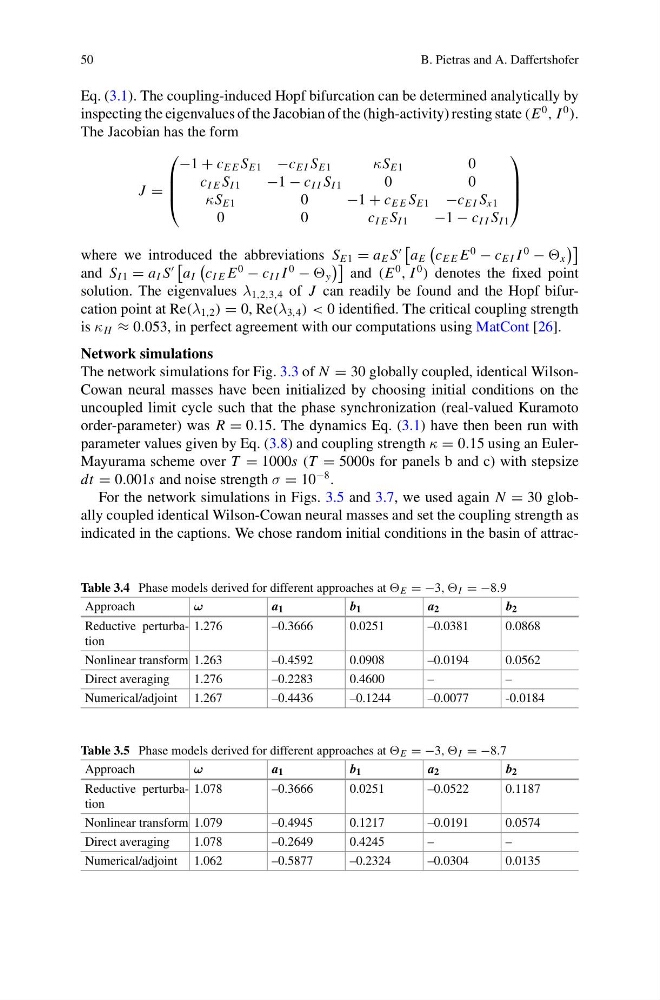
The Jacobian has the form
J =
⎛
⎜
⎜
⎝
−1 + c E E S E1 −c E I S E1
κS E1
0
c I E S I 1
−1 − c I I S I 1
0
0
κS E1
0
−1 + c E E S E1 −c E I S x1
0
0
c I E S I 1
−1 − c I I S I 1
⎞
⎟
⎟
⎠
where we introduced the abbreviations S E1 = a E S
a E
c E E E
0
− c E I I
0
− x
and S I 1 = a I S
a I
c I E E
0
− c I I I
0
− y
and (E
0
, I
0
) denotes the fixed point
solution. The eigenvalues λ 1,2,3,4 of J can readily be found and the Hopf bifurcation point at Re(λ 1,2 ) = 0, Re(λ 3,4 ) < 0 identified. The critical coupling strength
is κ H ≈ 0.053, in perfect agreement with our computations using MatCont [26].
Network simulations
The network simulations for Fig. 3.3 of N = 30 globally coupled, identical WilsonCowan neural masses have been initialized by choosing initial conditions on the
uncoupled limit cycle such that the phase synchronization (real-valued Kuramoto
order-parameter) was R = 0.15. The dynamics Eq. (3.1) have then been run with
parameter values given by Eq. (3.8) and coupling strength κ = 0.15 using an EulerMayurama scheme over T = 1000s (T = 5000s for panels b and c) with stepsize
dt = 0.001s and noise strength σ = 10
−8 .
For the network simulations in Figs. 3.5 and 3.7, we used again N = 30 globally coupled identical Wilson-Cowan neural masses and set the coupling strength as
indicated in the captions. We chose random initial conditions in the basin of attracTable 3.4 Phase models derived for different approaches at E = −3, , I = −8.9
Approach
ω
a 1
b 1
a 2
b 2
Reductive perturbation
1.276
–0.3666
0.0251
–0.0381
0.0868
Nonlinear transform 1.263
–0.4592
0.0908
–0.0194
0.0562
Direct averaging
1.276
–0.2283
0.4600
–
–
Numerical/adjoint 1.267
–0.4436
–0.1244
–0.0077
-0.0184
Table 3.5 Phase models derived for different approaches at E = −3, , I = −8.7
Approach
ω
a 1
b 1
a 2
b 2
Reductive perturbation
1.078
–0.3666
0.0251
–0.0522
0.1187
Nonlinear transform 1.079
–0.4945
0.1217
–0.0191
0.0574
Direct averaging
1.078
–0.2649
0.4245
–
–
Numerical/adjoint 1.062
–0.5877
–0.2324
–0.0304
0.0135
B. Pietras and A. Daffertshofer
Eq. (3.1). The coupling-induced Hopf bifurcation can be determined analytically by
inspecting the eigenvalues of the Jacobian of the (high-activity) resting state (E
0
, I
0
).
The Jacobian has the form
J =
⎛
⎜
⎜
⎝
−1 + c E E S E1 −c E I S E1
κS E1
0
c I E S I 1
−1 − c I I S I 1
0
0
κS E1
0
−1 + c E E S E1 −c E I S x1
0
0
c I E S I 1
−1 − c I I S I 1
⎞
⎟
⎟
⎠
where we introduced the abbreviations S E1 = a E S
a E
c E E E
0
− c E I I
0
− x
and S I 1 = a I S
a I
c I E E
0
− c I I I
0
− y
and (E
0
, I
0
) denotes the fixed point
solution. The eigenvalues λ 1,2,3,4 of J can readily be found and the Hopf bifurcation point at Re(λ 1,2 ) = 0, Re(λ 3,4 ) < 0 identified. The critical coupling strength
is κ H ≈ 0.053, in perfect agreement with our computations using MatCont [26].
Network simulations
The network simulations for Fig. 3.3 of N = 30 globally coupled, identical WilsonCowan neural masses have been initialized by choosing initial conditions on the
uncoupled limit cycle such that the phase synchronization (real-valued Kuramoto
order-parameter) was R = 0.15. The dynamics Eq. (3.1) have then been run with
parameter values given by Eq. (3.8) and coupling strength κ = 0.15 using an EulerMayurama scheme over T = 1000s (T = 5000s for panels b and c) with stepsize
dt = 0.001s and noise strength σ = 10
−8 .
For the network simulations in Figs. 3.5 and 3.7, we used again N = 30 globally coupled identical Wilson-Cowan neural masses and set the coupling strength as
indicated in the captions. We chose random initial conditions in the basin of attracTable 3.4 Phase models derived for different approaches at E = −3, , I = −8.9
Approach
ω
a 1
b 1
a 2
b 2
Reductive perturbation
1.276
–0.3666
0.0251
–0.0381
0.0868
Nonlinear transform 1.263
–0.4592
0.0908
–0.0194
0.0562
Direct averaging
1.276
–0.2283
0.4600
–
–
Numerical/adjoint 1.267
–0.4436
–0.1244
–0.0077
-0.0184
Table 3.5 Phase models derived for different approaches at E = −3, , I = −8.7
Approach
ω
a 1
b 1
a 2
b 2
Reductive perturbation
1.078
–0.3666
0.0251
–0.0522
0.1187
Nonlinear transform 1.079
–0.4945
0.1217
–0.0191
0.0574
Direct averaging
1.078
–0.2649
0.4245
–
–
Numerical/adjoint 1.062
–0.5877
–0.2324
–0.0304
0.0135