

3 Reduced Phase Models of Oscillatory Neural Networks
41
0
0.2
0.4
0.6
0.8
1
1.2
1.4
1.6
0
0.1
0.2
0.3
0.4
0.5
0.6
0.7
0.8
0.9
1
E
1,2
1.316 1.318 1.32 1.322
0.28
0.3
0.32
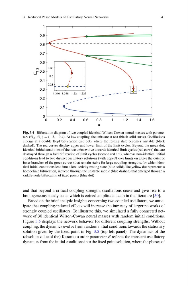
Fig. 3.4 Bifurcation diagram of two coupled identical Wilson-Cowan neural masses with parameters (( E , , I ) = (−3, −9.4). At low coupling, the units are at rest (black solid curve). Oscillations
emerge at a double Hopf bifurcation (red dot), where the resting state becomes unstable (black
dashed). The red curves display upper and lower limit of the limit cycles. Beyond the green dot,
identical initial conditions of the two units evolve towards identical limit cycles (red curve) that are
destroyed through a fold bifurcation of limit cycles (second red dot), whereas non-identical initial
conditions lead to two distinct oscillatory solutions (with upper/lower limits on either the outer or
inner branches of the green curves) that remain stable for large coupling strengths, for which identical initial conditions lead into a low-activity resting state (blue solid).The yellow dot represents a
homoclinic bifurcation, induced through the unstable saddle (blue dashed) that emerged through a
saddle-node bifurcation of fixed points (blue dot)
and that beyond a critical coupling strength, oscillations cease and give rise to a
homogeneous steady state, which is coined amplitude death in the literature [50].
Based on the brief analytic insights concerning two coupled oscillators, we anticipate that coupling-induced effects will increase the intricacy of larger networks of
strongly coupled oscillators. To illustrate this, we simulated a fully connected network of 30 identical Wilson-Cowan neural masses with random initial conditions.
Figure 3.5 displays the network behavior for different coupling strengths. Without
coupling, the dynamics evolve from random initial conditions towards the stationary
solution given by the fixed point in Fig. 3.5 (top left panel). The dynamics of the
(absolute value of the) Kuramoto order parameter R reflects the transient oscillatory
dynamics from the initial conditions into the fixed point solution, where the phases of
41
0
0.2
0.4
0.6
0.8
1
1.2
1.4
1.6
0
0.1
0.2
0.3
0.4
0.5
0.6
0.7
0.8
0.9
1
E
1,2
1.316 1.318 1.32 1.322
0.28
0.3
0.32
Fig. 3.4 Bifurcation diagram of two coupled identical Wilson-Cowan neural masses with parameters (( E , , I ) = (−3, −9.4). At low coupling, the units are at rest (black solid curve). Oscillations
emerge at a double Hopf bifurcation (red dot), where the resting state becomes unstable (black
dashed). The red curves display upper and lower limit of the limit cycles. Beyond the green dot,
identical initial conditions of the two units evolve towards identical limit cycles (red curve) that are
destroyed through a fold bifurcation of limit cycles (second red dot), whereas non-identical initial
conditions lead to two distinct oscillatory solutions (with upper/lower limits on either the outer or
inner branches of the green curves) that remain stable for large coupling strengths, for which identical initial conditions lead into a low-activity resting state (blue solid).The yellow dot represents a
homoclinic bifurcation, induced through the unstable saddle (blue dashed) that emerged through a
saddle-node bifurcation of fixed points (blue dot)
and that beyond a critical coupling strength, oscillations cease and give rise to a
homogeneous steady state, which is coined amplitude death in the literature [50].
Based on the brief analytic insights concerning two coupled oscillators, we anticipate that coupling-induced effects will increase the intricacy of larger networks of
strongly coupled oscillators. To illustrate this, we simulated a fully connected network of 30 identical Wilson-Cowan neural masses with random initial conditions.
Figure 3.5 displays the network behavior for different coupling strengths. Without
coupling, the dynamics evolve from random initial conditions towards the stationary
solution given by the fixed point in Fig. 3.5 (top left panel). The dynamics of the
(absolute value of the) Kuramoto order parameter R reflects the transient oscillatory
dynamics from the initial conditions into the fixed point solution, where the phases of