

406
Y. A. Abdulhameed et al.
26.3 Analysis of Cardiovascular Time Series
Prior to analysis, time-series were inspected in order to detect any apparent anomalies,
e.g. movement artefacts or rhythmic patterns clearly different from the blood flow
oscillations of interest. Such effects might be expected to stem from methodological
or physiological factors including poor electrode placement or poor electrical contact
due e.g. to dry skin. The intention was that time series that were demonstrably
defective would be discarded. In practice, this occurred only once: data from one
febrile malaria patient were removed from the data set on account of a defective
respiratory signal, seemingly because the respiratory belt had not been properly
fastened around the patient’s thorax.
26.3.1 Spectral Analysis
Traditionally, representations of time series in the frequency domain are obtained
with the fast Fourier transform, which constitutes a periodic function in terms of
sines and cosines. This makes it suitable for analysing time series whose components
are strictly periodic in nature, but it is unsuitable for LDF blood flow signals whose
spectral content is inherently non-periodic. Although the limitations of the Fourier
transform can partially be addressed by dividing the time series into shorter timewindows within which there is not much time variation, a better way forward is by
the use of wavelet analysis [38] which, by using an adaptive window length that
simultaneously analyses time series at each moment in time, provides both optimal
frequency resolution and time localisation [8, 14].
Wavelet analysis is a scale-independent method comprising an adaptive window
length allowing low frequencies to be analysed using longer wavelets, and higher
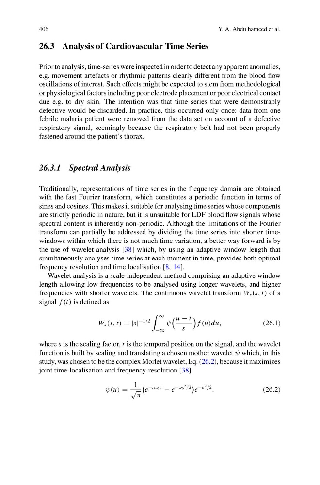
frequencies with shorter wavelets. The continuous wavelet transform W s (s, t) of a
signal f (t) is defined as
W s (s, t) = |s|
−1/2
∞
−∞
ψ
u − t
s
f (u)du,
(26.1)
where s is the scaling factor, t is the temporal position on the signal, and the wavelet
function is built by scaling and translating a chosen mother wavelet ψ which, in this
study, was chosen to be the complex Morlet wavelet, Eq. (26.2), because it maximizes
joint time-localisation and frequency-resolution [38]
ψ(u) =
1
√
π
e
−iω 0 u
− e
−ω 0
2 /2
e
−u
2 /2
.
(26.2)
Y. A. Abdulhameed et al.
26.3 Analysis of Cardiovascular Time Series
Prior to analysis, time-series were inspected in order to detect any apparent anomalies,
e.g. movement artefacts or rhythmic patterns clearly different from the blood flow
oscillations of interest. Such effects might be expected to stem from methodological
or physiological factors including poor electrode placement or poor electrical contact
due e.g. to dry skin. The intention was that time series that were demonstrably
defective would be discarded. In practice, this occurred only once: data from one
febrile malaria patient were removed from the data set on account of a defective
respiratory signal, seemingly because the respiratory belt had not been properly
fastened around the patient’s thorax.
26.3.1 Spectral Analysis
Traditionally, representations of time series in the frequency domain are obtained
with the fast Fourier transform, which constitutes a periodic function in terms of
sines and cosines. This makes it suitable for analysing time series whose components
are strictly periodic in nature, but it is unsuitable for LDF blood flow signals whose
spectral content is inherently non-periodic. Although the limitations of the Fourier
transform can partially be addressed by dividing the time series into shorter timewindows within which there is not much time variation, a better way forward is by
the use of wavelet analysis [38] which, by using an adaptive window length that
simultaneously analyses time series at each moment in time, provides both optimal
frequency resolution and time localisation [8, 14].
Wavelet analysis is a scale-independent method comprising an adaptive window
length allowing low frequencies to be analysed using longer wavelets, and higher
frequencies with shorter wavelets. The continuous wavelet transform W s (s, t) of a
signal f (t) is defined as
W s (s, t) = |s|
−1/2
∞
−∞
ψ
u − t
s
f (u)du,
(26.1)
where s is the scaling factor, t is the temporal position on the signal, and the wavelet
function is built by scaling and translating a chosen mother wavelet ψ which, in this
study, was chosen to be the complex Morlet wavelet, Eq. (26.2), because it maximizes
joint time-localisation and frequency-resolution [38]
ψ(u) =
1
√
π
e
−iω 0 u
− e
−ω 0
2 /2
e
−u
2 /2
.
(26.2)