

20
H. Nakao
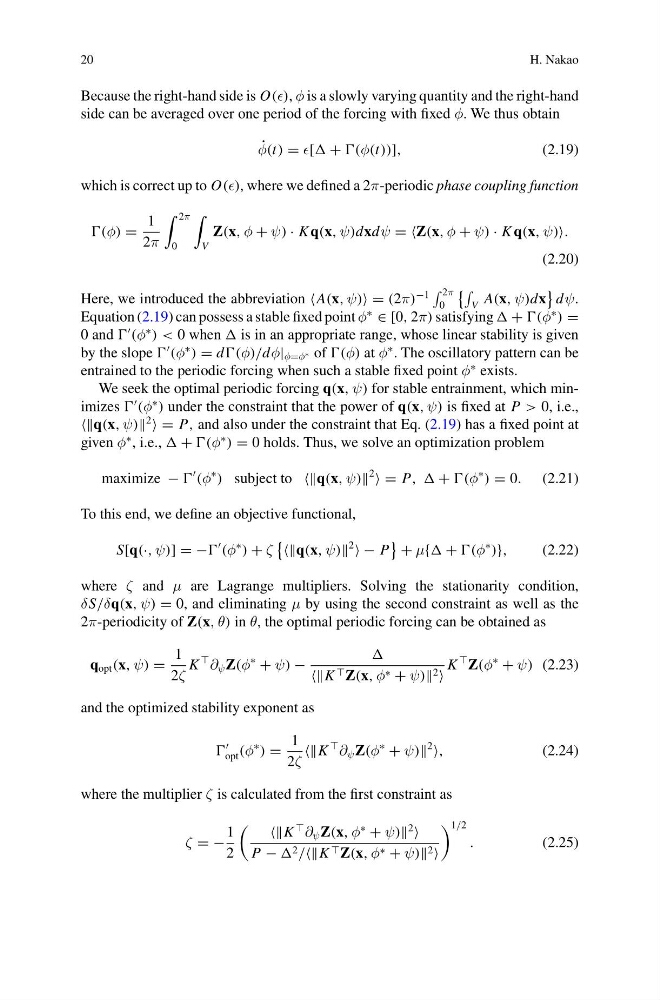
Because the right-hand side is O(), φ is a slowly varying quantity and the right-hand
side can be averaged over one period of the forcing with fixed φ. We thus obtain
˙
φ(t) = [ + (φ(t))],
(2.19)
which is correct up to O(), where we defined a 2π-periodic phase coupling function
(φ) =
1
2π
2π
0
V
Z(x, φ + ψ) · K q(x, ψ)dxdψ = =Z(x, φ + ψ) · K q(x, ψ).
(2.20)
Here, we introduced the abbreviation A(x, ψ) = (2π)
−1
2π
0
V A(x, ψ)dx
dψ.
Equation (2.19) can possess a stable fixed point φ
∗
∈ [0, 2π) satisfying + (φ
∗
) =
0 and
(φ
∗
) < 0 when is in an appropriate range, whose linear stability is given
by the slope
(φ
∗
) = d(φ)/dφ| φ=φ ∗ of (φ) at φ
∗ . The oscillatory pattern can be
entrained to the periodic forcing when such a stable fixed point φ
∗ exists.
We seek the optimal periodic forcing q(x, ψ) for stable entrainment, which minimizes
(φ
∗
) under the constraint that the power of q(x, ψ) is fixed at P > 0, i.e.,
q(x, ψ)
2
= P, and also under the constraint that Eq. (2.19) has a fixed point at
given φ
∗ , i.e., + (φ
∗
) = 0 holds. Thus, we solve an optimization problem
maximize −
(φ
∗
) subject to q(x, ψ)
2
= P, , + (φ
∗
) = 0. (2.21)
To this end, we define an objective functional,
S[q(·, ψ)] = −
(φ
∗
) + ζ
q(x, ψ)
2
− P
+ μ{ + (φ
∗
)},
(2.22)
where ζ and μ are Lagrange multipliers. Solving the stationarity condition,
δS/δq(x, ψ) = 0, and eliminating μ by using the second constraint as well as the
2π-periodicity of Z(x, θ) in θ, the optimal periodic forcing can be obtained as
q opt (x, ψ) =
1
2ζ
K
∂ ψ Z(φ
∗
+ ψ) −
K Z(x, φ ∗ + ψ) 2
K
Z(φ
∗
+ ψ) (2.23)
and the optimized stability exponent as
opt (φ
∗
) =
1
2ζ
K
∂ ψ Z(φ
∗
+ ψ)
2
,
(2.24)
where the multiplier ζ is calculated from the first constraint as
ζ = −
1
2
K
∂ ψ Z(x, φ
∗
+ ψ)
2
P − 2 /K Z(x, φ ∗ + ψ) 2
1/2
.
(2.25)
H. Nakao
Because the right-hand side is O(), φ is a slowly varying quantity and the right-hand
side can be averaged over one period of the forcing with fixed φ. We thus obtain
˙
φ(t) = [ + (φ(t))],
(2.19)
which is correct up to O(), where we defined a 2π-periodic phase coupling function
(φ) =
1
2π
2π
0
V
Z(x, φ + ψ) · K q(x, ψ)dxdψ = =Z(x, φ + ψ) · K q(x, ψ).
(2.20)
Here, we introduced the abbreviation A(x, ψ) = (2π)
−1
2π
0
V A(x, ψ)dx
dψ.
Equation (2.19) can possess a stable fixed point φ
∗
∈ [0, 2π) satisfying + (φ
∗
) =
0 and
(φ
∗
) < 0 when is in an appropriate range, whose linear stability is given
by the slope
(φ
∗
) = d(φ)/dφ| φ=φ ∗ of (φ) at φ
∗ . The oscillatory pattern can be
entrained to the periodic forcing when such a stable fixed point φ
∗ exists.
We seek the optimal periodic forcing q(x, ψ) for stable entrainment, which minimizes
(φ
∗
) under the constraint that the power of q(x, ψ) is fixed at P > 0, i.e.,
q(x, ψ)
2
= P, and also under the constraint that Eq. (2.19) has a fixed point at
given φ
∗ , i.e., + (φ
∗
) = 0 holds. Thus, we solve an optimization problem
maximize −
(φ
∗
) subject to q(x, ψ)
2
= P, , + (φ
∗
) = 0. (2.21)
To this end, we define an objective functional,
S[q(·, ψ)] = −
(φ
∗
) + ζ
q(x, ψ)
2
− P
+ μ{ + (φ
∗
)},
(2.22)
where ζ and μ are Lagrange multipliers. Solving the stationarity condition,
δS/δq(x, ψ) = 0, and eliminating μ by using the second constraint as well as the
2π-periodicity of Z(x, θ) in θ, the optimal periodic forcing can be obtained as
q opt (x, ψ) =
1
2ζ
K
∂ ψ Z(φ
∗
+ ψ) −
K Z(x, φ ∗ + ψ) 2
K
Z(φ
∗
+ ψ) (2.23)
and the optimized stability exponent as
opt (φ
∗
) =
1
2ζ
K
∂ ψ Z(φ
∗
+ ψ)
2
,
(2.24)
where the multiplier ζ is calculated from the first constraint as
ζ = −
1
2
K
∂ ψ Z(x, φ
∗
+ ψ)
2
P − 2 /K Z(x, φ ∗ + ψ) 2
1/2
.
(2.25)