

18
H. Nakao
Though it is difficult to obtain the functionals and R explicitly, it can be shown
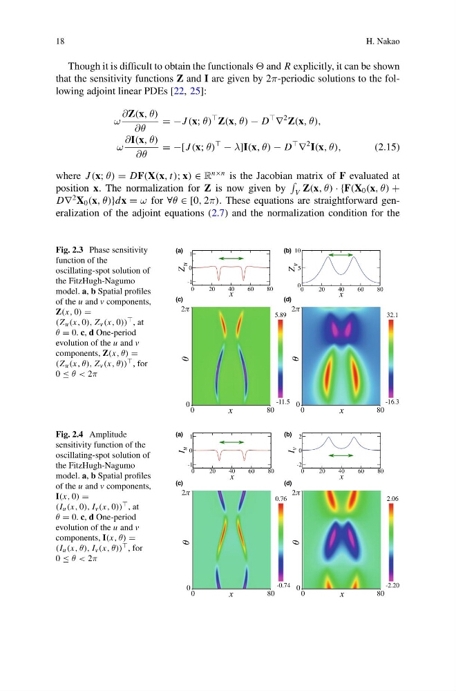
that the sensitivity functions Z and I are given by 2π-periodic solutions to the following adjoint linear PDEs [22, 25]:
ω
∂Z(x, θ)
∂θ
= −J (x; θ)
Z(x, θ) − D
∇
2 Z(x, θ),
ω
∂I(x, θ)
∂θ
= −[J (x; θ)
− λ]I(x, θ) − D
∇
2 I(x, θ),
(2.15)
where J (x; θ) = DF(X(x, t); x) ∈ R
n×n is the Jacobian matrix of F evaluated at
position x. The normalization for Z is now given by
V Z(x, θ) · {F(X 0 (x, θ) +
D∇
2 X 0 (x, θ)}dx = ω for ∀θ ∈ [0, 2π). These equations are straightforward generalization of the adjoint equations (2.7) and the normalization condition for the
Fig. 2.3 Phase sensitivity
function of the
oscillating-spot solution of
the FitzHugh-Nagumo
model. a, b Spatial profiles
of the u and v components,
Z(x, 0) =
(Z u (x, 0), Z v (x, 0)) , at
θ = 0. c, d One-period
evolution of the u and v
components, Z(x, θ) =
(Z u (x, θ), Z v (x, θ)) , for
0 ≤ θ < 2π
(a)
(b)
(c)
(d)
5.89
-11.5
32.1
-16.3
2
0
0
80
0
80
0
2
x
x
60
80
x
-1
0
1
Z
u
0
2 0
4 0
0
2 0
4 0
60
80
x
0
5
10
Z
v
Fig. 2.4 Amplitude
sensitivity function of the
oscillating-spot solution of
the FitzHugh-Nagumo
model. a, b Spatial profiles
of the u and v components,
I(x, 0) =
(I u (x, 0), I v (x, 0)) , at
θ = 0. c, d One-period
evolution of the u and v
components, I(x, θ) =
(I u (x, θ), I v (x, θ)) , for
0 ≤ θ < 2π
(a)
(b)
(c)
(d)
0.76
-0.74
2.06
-2.20
2
0
0
80
0
80
0
2
x
x
60
80
x
-1
0
1
I
u
0
2 0
4 0
0
2 0
4 0
60
80
x
-2
0
2
I
v
H. Nakao
Though it is difficult to obtain the functionals and R explicitly, it can be shown
that the sensitivity functions Z and I are given by 2π-periodic solutions to the following adjoint linear PDEs [22, 25]:
ω
∂Z(x, θ)
∂θ
= −J (x; θ)
Z(x, θ) − D
∇
2 Z(x, θ),
ω
∂I(x, θ)
∂θ
= −[J (x; θ)
− λ]I(x, θ) − D
∇
2 I(x, θ),
(2.15)
where J (x; θ) = DF(X(x, t); x) ∈ R
n×n is the Jacobian matrix of F evaluated at
position x. The normalization for Z is now given by
V Z(x, θ) · {F(X 0 (x, θ) +
D∇
2 X 0 (x, θ)}dx = ω for ∀θ ∈ [0, 2π). These equations are straightforward generalization of the adjoint equations (2.7) and the normalization condition for the
Fig. 2.3 Phase sensitivity
function of the
oscillating-spot solution of
the FitzHugh-Nagumo
model. a, b Spatial profiles
of the u and v components,
Z(x, 0) =
(Z u (x, 0), Z v (x, 0)) , at
θ = 0. c, d One-period
evolution of the u and v
components, Z(x, θ) =
(Z u (x, θ), Z v (x, θ)) , for
0 ≤ θ < 2π
(a)
(b)
(c)
(d)
5.89
-11.5
32.1
-16.3
2
0
0
80
0
80
0
2
x
x
60
80
x
-1
0
1
Z
u
0
2 0
4 0
0
2 0
4 0
60
80
x
0
5
10
Z
v
Fig. 2.4 Amplitude
sensitivity function of the
oscillating-spot solution of
the FitzHugh-Nagumo
model. a, b Spatial profiles
of the u and v components,
I(x, 0) =
(I u (x, 0), I v (x, 0)) , at
θ = 0. c, d One-period
evolution of the u and v
components, I(x, θ) =
(I u (x, θ), I v (x, θ)) , for
0 ≤ θ < 2π
(a)
(b)
(c)
(d)
0.76
-0.74
2.06
-2.20
2
0
0
80
0
80
0
2
x
x
60
80
x
-1
0
1
I
u
0
2 0
4 0
0
2 0
4 0
60
80
x
-2
0
2
I
v