

12 Phase Reconstruction with Iterated Hilbert Transforms
199
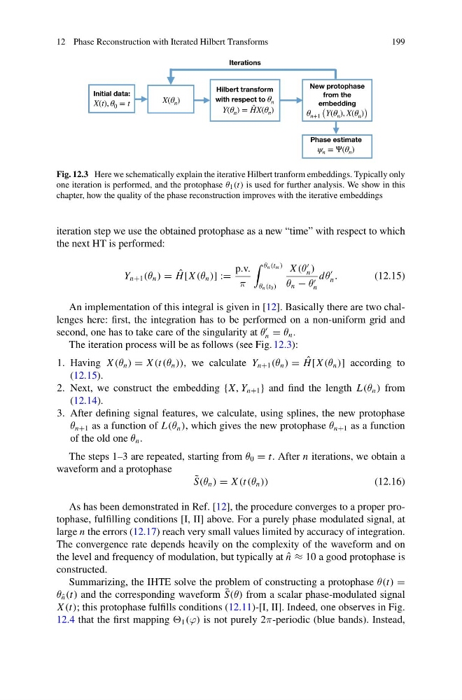
Fig. 12.3 Here we schematically explain the iterative Hilbert tranform embeddings. Typically only
one iteration is performed, and the protophase θ 1 (t) is used for further analysis. We show in this
chapter, how the quality of the phase reconstruction improves with the iterative embeddings
iteration step we use the obtained protophase as a new “time” with respect to which
the next HT is performed:
Y n+1 (θ n ) = ˆ
H [X (θ n )] :=
p.v.
π
θ n (t m )
θ n (t 0 )
X (θ
n )
θ n − θ
n
dθ
n .
(12.15)
An implementation of this integral is given in [12]. Basically there are two challenges here: first, the integration has to be performed on a non-uniform grid and
second, one has to take care of the singularity at θ
n = θ n .
The iteration process will be as follows (see Fig. 12.3):
1. Having X (θ n ) = X (t (θ n )), we calculate Y n+1 (θ n ) = ˆ
H [X (θ n )] according to
(12.15).
2. Next, we construct the embedding {X, Y n+1 } and find the length L(θ n ) from
(12.14).
3. After defining signal features, we calculate, using splines, the new protophase
θ n+1 as a function of L(θ n ), which gives the new protophase θ n+1 as a function
of the old one θ n .
The steps 1–3 are repeated, starting from θ 0 = t. After n iterations, we obtain a
waveform and a protophase
˜
S(θ n ) = X (t (θ n ))
(12.16)
As has been demonstrated in Ref. [12], the procedure converges to a proper protophase, fulfilling conditions [I, II] above. For a purely phase modulated signal, at
large n the errors (12.17) reach very small values limited by accuracy of integration.
The convergence rate depends heavily on the complexity of the waveform and on
the level and frequency of modulation, but typically at ˆ
n ≈ 10 a good protophase is
constructed.
Summarizing, the IHTE solve the problem of constructing a protophase θ(t) =
θ ˆ
n (t) and the corresponding waveform ˜
S(θ) from a scalar phase-modulated signal
X (t); this protophase fulfills conditions (12.11)-[I, II]. Indeed, one observes in Fig.
12.4 that the first mapping 1 (ϕ) is not purely 2π-periodic (blue bands). Instead,
199
Fig. 12.3 Here we schematically explain the iterative Hilbert tranform embeddings. Typically only
one iteration is performed, and the protophase θ 1 (t) is used for further analysis. We show in this
chapter, how the quality of the phase reconstruction improves with the iterative embeddings
iteration step we use the obtained protophase as a new “time” with respect to which
the next HT is performed:
Y n+1 (θ n ) = ˆ
H [X (θ n )] :=
p.v.
π
θ n (t m )
θ n (t 0 )
X (θ
n )
θ n − θ
n
dθ
n .
(12.15)
An implementation of this integral is given in [12]. Basically there are two challenges here: first, the integration has to be performed on a non-uniform grid and
second, one has to take care of the singularity at θ
n = θ n .
The iteration process will be as follows (see Fig. 12.3):
1. Having X (θ n ) = X (t (θ n )), we calculate Y n+1 (θ n ) = ˆ
H [X (θ n )] according to
(12.15).
2. Next, we construct the embedding {X, Y n+1 } and find the length L(θ n ) from
(12.14).
3. After defining signal features, we calculate, using splines, the new protophase
θ n+1 as a function of L(θ n ), which gives the new protophase θ n+1 as a function
of the old one θ n .
The steps 1–3 are repeated, starting from θ 0 = t. After n iterations, we obtain a
waveform and a protophase
˜
S(θ n ) = X (t (θ n ))
(12.16)
As has been demonstrated in Ref. [12], the procedure converges to a proper protophase, fulfilling conditions [I, II] above. For a purely phase modulated signal, at
large n the errors (12.17) reach very small values limited by accuracy of integration.
The convergence rate depends heavily on the complexity of the waveform and on
the level and frequency of modulation, but typically at ˆ
n ≈ 10 a good protophase is
constructed.
Summarizing, the IHTE solve the problem of constructing a protophase θ(t) =
θ ˆ
n (t) and the corresponding waveform ˜
S(θ) from a scalar phase-modulated signal
X (t); this protophase fulfills conditions (12.11)-[I, II]. Indeed, one observes in Fig.
12.4 that the first mapping 1 (ϕ) is not purely 2π-periodic (blue bands). Instead,