

12 Phase Reconstruction with Iterated Hilbert Transforms
195
data analysis, one faces a problem of the phase dynamics reconstruction solely from
the observations of a driven oscillator. From the time series of a scalar observable,
one wants to reconstruct the phase dynamics equation (12.2).
The first assumption we make is that the phase modulation of the process observed
is much stronger than the amplitude modulation. Although, according to the theory,
amplitude perturbations appear already in the leading order ∼ ε (cf. Eq. (12.5)),
these variations could be small if the stability of the limit cycle is strong. Indeed, like
example Eq. (12.5) shows, perturbations of the amplitude are inverse proportional to
the stability of the limit cycle ∼ ε/μ, and are additionally small for μ large. Thus, for
the rest of this chapter we assume that the dynamical process under reconstruction
is solely determined by the dynamics of the phase.
Generally, a time series emanates from an observable X [y(t)] of the systems
dynamics. According to the assumption above, we neglect amplitude modulation
which means that we assume y = y 0 , so that the scalar signal observed is purely
phase modulated
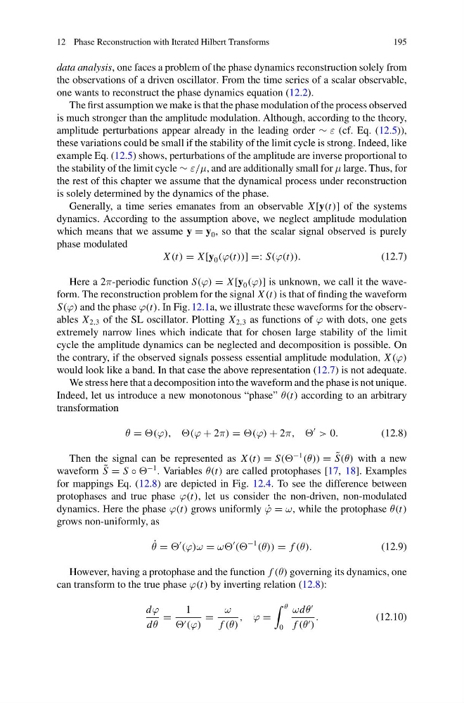
X (t) = X [y 0 (ϕ(t))] =: S(ϕ(t)).
(12.7)
Here a 2π-periodic function S(ϕ) = X [y 0 (ϕ)] is unknown, we call it the waveform. The reconstruction problem for the signal X (t) is that of finding the waveform
S(ϕ) and the phase ϕ(t). In Fig. 12.1a, we illustrate these waveforms for the observables X 2,3 of the SL oscillator. Plotting X 2,3 as functions of ϕ with dots, one gets
extremely narrow lines which indicate that for chosen large stability of the limit
cycle the amplitude dynamics can be neglected and decomposition is possible. On
the contrary, if the observed signals possess essential amplitude modulation, X (ϕ)
would look like a band. In that case the above representation (12.7) is not adequate.
We stress here that a decomposition into the waveform and the phase is not unique.
Indeed, let us introduce a new monotonous “phase” θ(t) according to an arbitrary
transformation
θ = (ϕ), ,(ϕ + 2π) = (ϕ) + 2π, ,
> 0.
(12.8)
Then the signal can be represented as X (t) = S((
−1
(θ)) = ˜
S(θ) with a new
waveform ˜
S = S ◦
−1 . Variables θ(t) are called protophases [17, 18]. Examples
for mappings Eq. (12.8) are depicted in Fig. 12.4. To see the difference between
protophases and true phase ϕ(t), let us consider the non-driven, non-modulated
dynamics. Here the phase ϕ(t) grows uniformly ˙
ϕ = ω, while the protophase θ(t)
grows non-uniformly, as
˙
θ =
(ϕ)ω = ω
((
−1
(θ)) = f (θ).
(12.9)
However, having a protophase and the function f (θ) governing its dynamics, one
can transform to the true phase ϕ(t) by inverting relation (12.8):
dϕ
dθ
=
1
(ϕ)
=
ω
f (θ)
, ϕ =
θ
0
ωdθ
f (θ )
.
(12.10)
195
data analysis, one faces a problem of the phase dynamics reconstruction solely from
the observations of a driven oscillator. From the time series of a scalar observable,
one wants to reconstruct the phase dynamics equation (12.2).
The first assumption we make is that the phase modulation of the process observed
is much stronger than the amplitude modulation. Although, according to the theory,
amplitude perturbations appear already in the leading order ∼ ε (cf. Eq. (12.5)),
these variations could be small if the stability of the limit cycle is strong. Indeed, like
example Eq. (12.5) shows, perturbations of the amplitude are inverse proportional to
the stability of the limit cycle ∼ ε/μ, and are additionally small for μ large. Thus, for
the rest of this chapter we assume that the dynamical process under reconstruction
is solely determined by the dynamics of the phase.
Generally, a time series emanates from an observable X [y(t)] of the systems
dynamics. According to the assumption above, we neglect amplitude modulation
which means that we assume y = y 0 , so that the scalar signal observed is purely
phase modulated
X (t) = X [y 0 (ϕ(t))] =: S(ϕ(t)).
(12.7)
Here a 2π-periodic function S(ϕ) = X [y 0 (ϕ)] is unknown, we call it the waveform. The reconstruction problem for the signal X (t) is that of finding the waveform
S(ϕ) and the phase ϕ(t). In Fig. 12.1a, we illustrate these waveforms for the observables X 2,3 of the SL oscillator. Plotting X 2,3 as functions of ϕ with dots, one gets
extremely narrow lines which indicate that for chosen large stability of the limit
cycle the amplitude dynamics can be neglected and decomposition is possible. On
the contrary, if the observed signals possess essential amplitude modulation, X (ϕ)
would look like a band. In that case the above representation (12.7) is not adequate.
We stress here that a decomposition into the waveform and the phase is not unique.
Indeed, let us introduce a new monotonous “phase” θ(t) according to an arbitrary
transformation
θ = (ϕ), ,(ϕ + 2π) = (ϕ) + 2π, ,
> 0.
(12.8)
Then the signal can be represented as X (t) = S((
−1
(θ)) = ˜
S(θ) with a new
waveform ˜
S = S ◦
−1 . Variables θ(t) are called protophases [17, 18]. Examples
for mappings Eq. (12.8) are depicted in Fig. 12.4. To see the difference between
protophases and true phase ϕ(t), let us consider the non-driven, non-modulated
dynamics. Here the phase ϕ(t) grows uniformly ˙
ϕ = ω, while the protophase θ(t)
grows non-uniformly, as
˙
θ =
(ϕ)ω = ω
((
−1
(θ)) = f (θ).
(12.9)
However, having a protophase and the function f (θ) governing its dynamics, one
can transform to the true phase ϕ(t) by inverting relation (12.8):
dϕ
dθ
=
1
(ϕ)
=
ω
f (θ)
, ϕ =
θ
0
ωdθ
f (θ )
.
(12.10)