

10 Useful Transformations from Non-autonomous to Autonomous Systems
167
h p
v (mV)
Stable
equilibrium
Stable periodic
Stable
equilibrium
h p
v (mV)
0
dt
dh p
0
dt
dh p
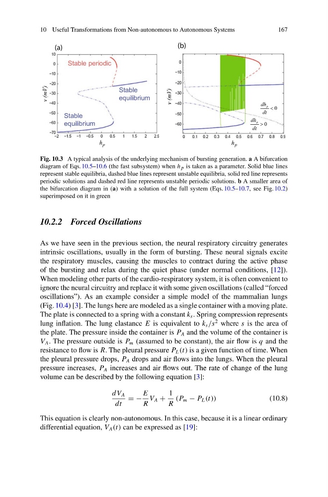
Fig. 10.3 A typical analysis of the underlying mechanism of bursting generation. a A bifurcation
diagram of Eqs. 10.5–10.6 (the fast subsystem) when h p is taken as a parameter. Solid blue lines
represent stable equilibria, dashed blue lines represent unstable equilibria, solid red line represents
periodic solutions and dashed red line represents unstable periodic solutions. b A smaller area of
the bifurcation diagram in (a) with a solution of the full system (Eqs. 10.5–10.7, see Fig.10.2)
superimposed on it in green
10.2.2 Forced Oscillations
As we have seen in the previous section, the neural respiratory circuitry generates
intrinsic oscillations, usually in the form of bursting. These neural signals excite
the respiratory muscles, causing the muscles to contract during the active phase
of the bursting and relax during the quiet phase (under normal conditions, [12]).
When modeling other parts of the cardio-respiratory system, it is often convenient to
ignore the neural circuitry and replace it with some given oscillations (called “forced
oscillations”). As an example consider a simple model of the mammalian lungs
(Fig. 10.4) [3]. The lungs here are modeled as a single container with a moving plate.
The plate is connected to a spring with a constant k s . Spring compression represents
lung inflation. The lung elastance E is equivalent to k s /s
2 where s is the area of
the plate. The pressure inside the container is P A and the volume of the container is
V A . The pressure outside is P m (assumed to be constant), the air flow is q and the
resistance to flow is R. The pleural pressure P L (t) is a given function of time. When
the pleural pressure drops, P A drops and air flows into the lungs. When the pleural
pressure increases, P A increases and air flows out. The rate of change of the lung
volume can be described by the following equation [3]:
dV A
dt
= −
E
R
V A +
1
R
(P m − P L (t))
(10.8)
This equation is clearly non-autonomous. In this case, because it is a linear ordinary
differential equation, V A (t) can be expressed as [19]:
167
h p
v (mV)
Stable
equilibrium
Stable periodic
Stable
equilibrium
h p
v (mV)
0
dt
dh p
0
dt
dh p
Fig. 10.3 A typical analysis of the underlying mechanism of bursting generation. a A bifurcation
diagram of Eqs. 10.5–10.6 (the fast subsystem) when h p is taken as a parameter. Solid blue lines
represent stable equilibria, dashed blue lines represent unstable equilibria, solid red line represents
periodic solutions and dashed red line represents unstable periodic solutions. b A smaller area of
the bifurcation diagram in (a) with a solution of the full system (Eqs. 10.5–10.7, see Fig.10.2)
superimposed on it in green
10.2.2 Forced Oscillations
As we have seen in the previous section, the neural respiratory circuitry generates
intrinsic oscillations, usually in the form of bursting. These neural signals excite
the respiratory muscles, causing the muscles to contract during the active phase
of the bursting and relax during the quiet phase (under normal conditions, [12]).
When modeling other parts of the cardio-respiratory system, it is often convenient to
ignore the neural circuitry and replace it with some given oscillations (called “forced
oscillations”). As an example consider a simple model of the mammalian lungs
(Fig. 10.4) [3]. The lungs here are modeled as a single container with a moving plate.
The plate is connected to a spring with a constant k s . Spring compression represents
lung inflation. The lung elastance E is equivalent to k s /s
2 where s is the area of
the plate. The pressure inside the container is P A and the volume of the container is
V A . The pressure outside is P m (assumed to be constant), the air flow is q and the
resistance to flow is R. The pleural pressure P L (t) is a given function of time. When
the pleural pressure drops, P A drops and air flows into the lungs. When the pleural
pressure increases, P A increases and air flows out. The rate of change of the lung
volume can be described by the following equation [3]:
dV A
dt
= −
E
R
V A +
1
R
(P m − P L (t))
(10.8)
This equation is clearly non-autonomous. In this case, because it is a linear ordinary
differential equation, V A (t) can be expressed as [19]: