

120
J. M. I. Newman et al.
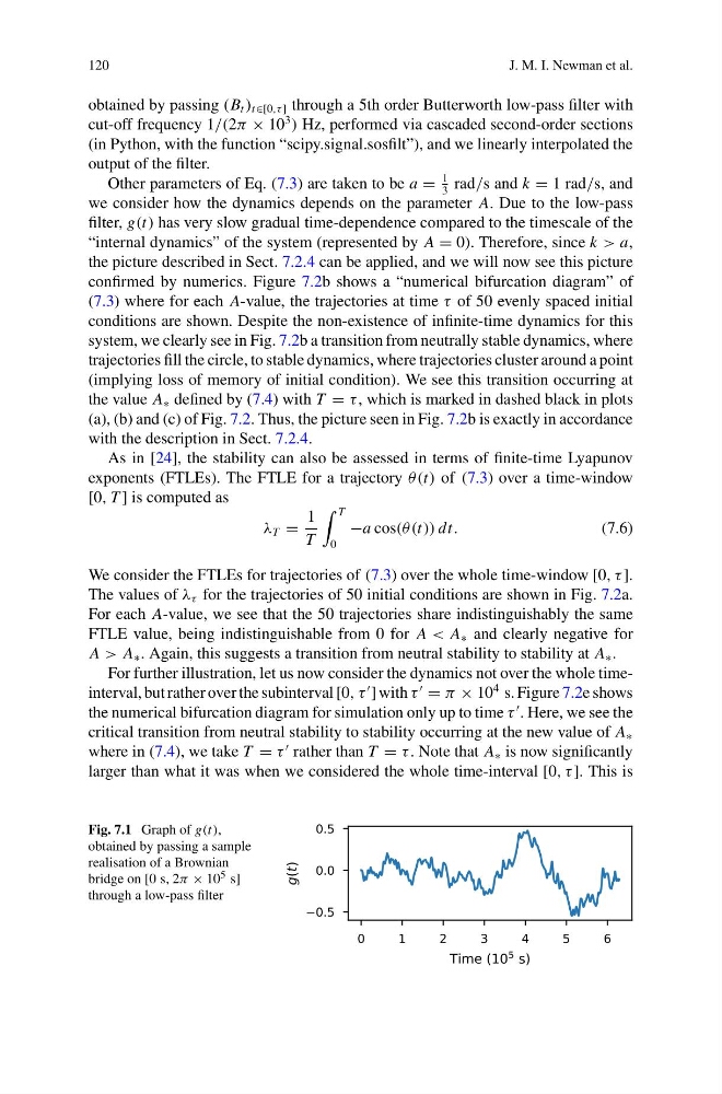
obtained by passing (B t ) t∈[0,τ ] through a 5th order Butterworth low-pass filter with
cut-off frequency 1/(2π × 10
3
) Hz, performed via cascaded second-order sections
(in Python, with the function “scipy.signal.sosfilt”), and we linearly interpolated the
output of the filter.
Other parameters of Eq. (7.3) are taken to be a =
1
3
rad/s and k = 1 rad/s, and
we consider how the dynamics depends on the parameter A. Due to the low-pass
filter, g(t) has very slow gradual time-dependence compared to the timescale of the
“internal dynamics” of the system (represented by A = 0). Therefore, since k > a,
the picture described in Sect. 7.2.4 can be applied, and we will now see this picture
confirmed by numerics. Figure 7.2b shows a “numerical bifurcation diagram” of
(7.3) where for each A-value, the trajectories at time τ of 50 evenly spaced initial
conditions are shown. Despite the non-existence of infinite-time dynamics for this
system, we clearly see in Fig. 7.2b a transition from neutrally stable dynamics, where
trajectories fill the circle, to stable dynamics, where trajectories cluster around a point
(implying loss of memory of initial condition). We see this transition occurring at
the value A ∗ defined by (7.4) with T = τ , which is marked in dashed black in plots
(a), (b) and (c) of Fig. 7.2. Thus, the picture seen in Fig. 7.2b is exactly in accordance
with the description in Sect. 7.2.4.
As in [24], the stability can also be assessed in terms of finite-time Lyapunov
exponents (FTLEs). The FTLE for a trajectory θ(t) of (7.3) over a time-window
[0, T ] is computed as
λ T =
1
T
T
0
−a cos(θ (t)) dt.
(7.6)
We consider the FTLEs for trajectories of (7.3) over the whole time-window [0, τ ].
The values of λ τ for the trajectories of 50 initial conditions are shown in Fig. 7.2a.
For each A-value, we see that the 50 trajectories share indistinguishably the same
FTLE value, being indistinguishable from 0 for A < A ∗ and clearly negative for
A > A ∗ . Again, this suggests a transition from neutral stability to stability at A ∗ .
For further illustration, let us now consider the dynamics not over the whole timeinterval, but rather over the subinterval [0, τ
] with τ
= π × 10
4 s. Figure 7.2e shows
the numerical bifurcation diagram for simulation only up to time τ
. Here, we see the
critical transition from neutral stability to stability occurring at the new value of A ∗
where in (7.4), we take T = τ
rather than T = τ . Note that A ∗ is now significantly
larger than what it was when we considered the whole time-interval [0, τ ]. This is
Fig. 7.1 Graph of g(t),
obtained by passing a sample
realisation of a Brownian
bridge on [0 s, 2π × 10 5 s]
through a low-pass filter
J. M. I. Newman et al.
obtained by passing (B t ) t∈[0,τ ] through a 5th order Butterworth low-pass filter with
cut-off frequency 1/(2π × 10
3
) Hz, performed via cascaded second-order sections
(in Python, with the function “scipy.signal.sosfilt”), and we linearly interpolated the
output of the filter.
Other parameters of Eq. (7.3) are taken to be a =
1
3
rad/s and k = 1 rad/s, and
we consider how the dynamics depends on the parameter A. Due to the low-pass
filter, g(t) has very slow gradual time-dependence compared to the timescale of the
“internal dynamics” of the system (represented by A = 0). Therefore, since k > a,
the picture described in Sect. 7.2.4 can be applied, and we will now see this picture
confirmed by numerics. Figure 7.2b shows a “numerical bifurcation diagram” of
(7.3) where for each A-value, the trajectories at time τ of 50 evenly spaced initial
conditions are shown. Despite the non-existence of infinite-time dynamics for this
system, we clearly see in Fig. 7.2b a transition from neutrally stable dynamics, where
trajectories fill the circle, to stable dynamics, where trajectories cluster around a point
(implying loss of memory of initial condition). We see this transition occurring at
the value A ∗ defined by (7.4) with T = τ , which is marked in dashed black in plots
(a), (b) and (c) of Fig. 7.2. Thus, the picture seen in Fig. 7.2b is exactly in accordance
with the description in Sect. 7.2.4.
As in [24], the stability can also be assessed in terms of finite-time Lyapunov
exponents (FTLEs). The FTLE for a trajectory θ(t) of (7.3) over a time-window
[0, T ] is computed as
λ T =
1
T
T
0
−a cos(θ (t)) dt.
(7.6)
We consider the FTLEs for trajectories of (7.3) over the whole time-window [0, τ ].
The values of λ τ for the trajectories of 50 initial conditions are shown in Fig. 7.2a.
For each A-value, we see that the 50 trajectories share indistinguishably the same
FTLE value, being indistinguishable from 0 for A < A ∗ and clearly negative for
A > A ∗ . Again, this suggests a transition from neutral stability to stability at A ∗ .
For further illustration, let us now consider the dynamics not over the whole timeinterval, but rather over the subinterval [0, τ
] with τ
= π × 10
4 s. Figure 7.2e shows
the numerical bifurcation diagram for simulation only up to time τ
. Here, we see the
critical transition from neutral stability to stability occurring at the new value of A ∗
where in (7.4), we take T = τ
rather than T = τ . Note that A ∗ is now significantly
larger than what it was when we considered the whole time-interval [0, τ ]. This is
Fig. 7.1 Graph of g(t),
obtained by passing a sample
realisation of a Brownian
bridge on [0 s, 2π × 10 5 s]
through a low-pass filter