

96
M. Lucas et al.
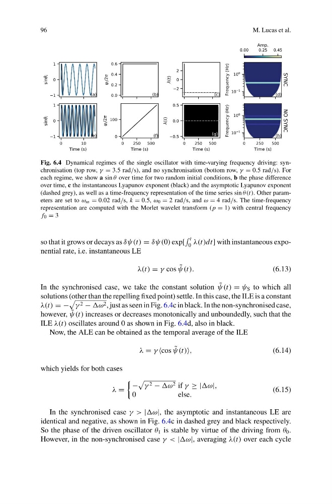
Fig. 6.4 Dynamical regimes of the single oscillator with time-varying frequency driving: synchronisation (top row, γ = 3.5 rad/s), and no synchronisation (bottom row, γ = 0.5 rad/s). For
each regime, we show a sin θ over time for two random initial conditions, b the phase difference
over time, c the instantaneous Lyapunov exponent (black) and the asymptotic Lyapunov exponent
(dashed grey), as well as a time-frequency representation of the time series sin θ(t). Other parameters are set to ω m = 0.02 rad/s, k = 0.5, ω 0 = 2 rad/s, and ω = 4 rad/s. The time-frequency
representation are computed with the Morlet wavelet transform ( p = 1) with central frequency
f 0 = 3
so that it grows or decays as δψ(t) = δψ(0) exp[
t
0 λ(t)dt] with instantaneous exponential rate, i.e. instantaneous LE
λ(t) = γ cos ˜
ψ(t).
(6.13)
In the synchronised case, we take the constant solution ˜
ψ(t) = ψ S to which all
solutions (other than the repelling fixed point) settle. In this case, the ILE is a constant
λ(t) = −
γ 2 − 2 , just as seen in Fig. 6.4c in black. In the non-synchronised case,
however, ˜
ψ(t) increases or decreases monotonically and unboundedly, such that the
ILE λ(t) oscillates around 0 as shown in Fig. 6.4d, also in black.
Now, the ALE can be obtained as the temporal average of the ILE
λ = γ cos ˜
ψ(t)
(6.14)
which yields for both cases
λ =
−
γ 2 − 2 if γ ≥ |
0
e l s e .
(6.15)
In the synchronised case γ > | the asymptotic and instantaneous LE are
identical and negative, as shown in Fig. 6.4c in dashed grey and black respectively.
So the phase of the driven oscillator θ 1 is stable by virtue of the driving from θ 0 .
However, in the non-synchronised case γ < | averaging λ(t) over each cycle
M. Lucas et al.
Fig. 6.4 Dynamical regimes of the single oscillator with time-varying frequency driving: synchronisation (top row, γ = 3.5 rad/s), and no synchronisation (bottom row, γ = 0.5 rad/s). For
each regime, we show a sin θ over time for two random initial conditions, b the phase difference
over time, c the instantaneous Lyapunov exponent (black) and the asymptotic Lyapunov exponent
(dashed grey), as well as a time-frequency representation of the time series sin θ(t). Other parameters are set to ω m = 0.02 rad/s, k = 0.5, ω 0 = 2 rad/s, and ω = 4 rad/s. The time-frequency
representation are computed with the Morlet wavelet transform ( p = 1) with central frequency
f 0 = 3
so that it grows or decays as δψ(t) = δψ(0) exp[
t
0 λ(t)dt] with instantaneous exponential rate, i.e. instantaneous LE
λ(t) = γ cos ˜
ψ(t).
(6.13)
In the synchronised case, we take the constant solution ˜
ψ(t) = ψ S to which all
solutions (other than the repelling fixed point) settle. In this case, the ILE is a constant
λ(t) = −
γ 2 − 2 , just as seen in Fig. 6.4c in black. In the non-synchronised case,
however, ˜
ψ(t) increases or decreases monotonically and unboundedly, such that the
ILE λ(t) oscillates around 0 as shown in Fig. 6.4d, also in black.
Now, the ALE can be obtained as the temporal average of the ILE
λ = γ cos ˜
ψ(t)
(6.14)
which yields for both cases
λ =
−
γ 2 − 2 if γ ≥ |
0
e l s e .
(6.15)
In the synchronised case γ > | the asymptotic and instantaneous LE are
identical and negative, as shown in Fig. 6.4c in dashed grey and black respectively.
So the phase of the driven oscillator θ 1 is stable by virtue of the driving from θ 0 .
However, in the non-synchronised case γ < | averaging λ(t) over each cycle