

6 Synchronisation and Non-autonomicity
95
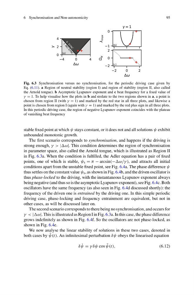
Fig. 6.3 Synchronisation versus no synchronisation, for the periodic driving case given by
Eq. (6.11). a Region of neutral stability (region I) and region of stability (region II, also called
the Arnold tongue). b Asymptotic Lyapunov exponent and c beat frequency for a fixed value of
γ = 1. To help visualise how the plots in b and crelate to the two regions shown in a, a point is
chosen from region II (with γ = 1) and marked by the red star in all three plots, and likewise a
point is chosen from region I (again with γ = 1) and marked by the red plus sign in all three plots.
In this periodic driving case, the region of negative Lyapunov exponent coincides with the plateau
of vanishing beat frequency
stable fixed point at which ψ stays constant, or it does not and all solutions ψ exhibit
unbounded monotonic growth.
The first scenario corresponds to synchronisation, and happens if the driving is
strong enough, γ > | This condition determines the region of synchronisation
in parameter space, also called the Arnold tongue, which is illustrated as Region II
in Fig. 6.3a. When the condition is fulfilled, the Adler equation has a pair of fixed
points, one of which is stable, ψ s = π − arcsin(− ), and attracts all initial
conditions apart from the unstable fixed point, see Fig. 6.4a. The phase difference ψ
thus settles on the constant value ψ s , as shown in Fig. 6.4b, and the driven oscillator is
thus phase-locked to the driving, with the instantaneous Lyapunov exponent always
being negative (and thus so is the asymptotic Lyapunov exponent), see Fig. 6.4c. Both
oscillators have the same frequency (as also seen in Fig. 6.4d discussed shortly): the
frequency of the driven one is entrained by the driving one. In this simple periodic
driving case, phase-locking and frequency entrainment are equivalent, but not in
other cases, as will be discussed later on.
The second scenario corresponds to there being no synchronisation, and occurs for
γ < | This is illustrated as Region I in Fig. 6.3a. In this case, the phase difference
grows indefinitely as shown in Fig. 6.4f. So the oscillators are not phase-locked, as
shown in Fig. 6.4e.
We now analyse the linear stability of solutions in these two cases, denoted in
both cases by ˜
ψ(t). An infinitesimal perturbation δψ obeys the linearised equation
δ ˙
ψ = γ δψ cos ˜
ψ(t),
(6.12)
95
Fig. 6.3 Synchronisation versus no synchronisation, for the periodic driving case given by
Eq. (6.11). a Region of neutral stability (region I) and region of stability (region II, also called
the Arnold tongue). b Asymptotic Lyapunov exponent and c beat frequency for a fixed value of
γ = 1. To help visualise how the plots in b and crelate to the two regions shown in a, a point is
chosen from region II (with γ = 1) and marked by the red star in all three plots, and likewise a
point is chosen from region I (again with γ = 1) and marked by the red plus sign in all three plots.
In this periodic driving case, the region of negative Lyapunov exponent coincides with the plateau
of vanishing beat frequency
stable fixed point at which ψ stays constant, or it does not and all solutions ψ exhibit
unbounded monotonic growth.
The first scenario corresponds to synchronisation, and happens if the driving is
strong enough, γ > | This condition determines the region of synchronisation
in parameter space, also called the Arnold tongue, which is illustrated as Region II
in Fig. 6.3a. When the condition is fulfilled, the Adler equation has a pair of fixed
points, one of which is stable, ψ s = π − arcsin(− ), and attracts all initial
conditions apart from the unstable fixed point, see Fig. 6.4a. The phase difference ψ
thus settles on the constant value ψ s , as shown in Fig. 6.4b, and the driven oscillator is
thus phase-locked to the driving, with the instantaneous Lyapunov exponent always
being negative (and thus so is the asymptotic Lyapunov exponent), see Fig. 6.4c. Both
oscillators have the same frequency (as also seen in Fig. 6.4d discussed shortly): the
frequency of the driven one is entrained by the driving one. In this simple periodic
driving case, phase-locking and frequency entrainment are equivalent, but not in
other cases, as will be discussed later on.
The second scenario corresponds to there being no synchronisation, and occurs for
γ < | This is illustrated as Region I in Fig. 6.3a. In this case, the phase difference
grows indefinitely as shown in Fig. 6.4f. So the oscillators are not phase-locked, as
shown in Fig. 6.4e.
We now analyse the linear stability of solutions in these two cases, denoted in
both cases by ˜
ψ(t). An infinitesimal perturbation δψ obeys the linearised equation
δ ˙
ψ = γ δψ cos ˜
ψ(t),
(6.12)