

6 Synchronisation and Non-autonomicity
89
Thus, non-autonomous systems are conceptually related to non-isolated systems
such as open systems: as illustrated in Fig. 6.1c, the system’s evolution depends on
its own internal dynamics but also on external influences, which can come in many
forms, as reflected in Eq. (6.2) by the explicit dependence of the evolution of x on t.
The formal study of non-autonomous dynamical systems started in the mathematical community [25] with early works on their stability including [1, 32,
38] and more recently [21]. Even though it is a much younger field than that of
autonomous dynamical systems, it started being used sparingly in other disciplines
such as physics [56] and biology [30]. In parallel, more and more researchers have
included time-variability in recent years, without necessarily using the word “nonautonomous” or its associated formalisms and methods. As an example, temporal
networks, i.e. networks with links that are time-dependent, have been applied successfully to diverse areas [19, 20].
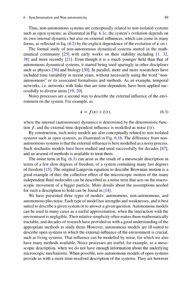
Noisy processes are a second way to describe the external influence of the environment on the system. For example, as
˙
x = f (x) + ξ(t),
(6.3)
where the internal (autonomous) dynamics is determined by the deterministic function f , and the external time-dependent influence is modelled as noise ξ(t).
By construction, such noisy models are also conceptually related to non-isolated
systems such as open systems, as illustrated in Fig. 6.1b. The difference from nonautonomous systems is that the external influence is here modelled as a noisy process.
Such stochastic models have been studied and used successfully for decades [47],
and an arsenal of methods is available to treat them.
The noise term in Eq. (6.3) can arise as the result of a mesoscale description in
terms of a few slow degrees of freedom, of a system containing many fast degrees
of freedom [15]. The original Langevin equation to describe Brownian motion is a
good example of this: the collective effect of the microscopic motion of the many
independent fluid molecules can be described as a noise term that acts on the macroscopic movement of a bigger particle. More details about the assumptions needed
for such a description to hold can be found in [14].
We have presented three types of models: autonomous, non-autonomous, and
autonomous plus noise. Each type of model has strengths and weaknesses, and is best
suited to describe a given system or to answer a given question. Autonomous models
can be used in many cases as a useful approximation, when the interaction with the
environment is negligible. Their relative simplicity often makes them mathematically
tractable, and decades of research have provided us with a good understanding of the
appropriate methods to study them. However, autonomous models are ill-suited to
describe open systems in which the external influence of the environment is crucial,
such as living systems. That influence can be modelled by noise, for which we also
have many methods available. Noisy processes are useful, for example, as a mesoscopic description, when we do not have enough information about the underlying
microscopic mechanisms. When possible, non-autonomous models of open systems
provide us with a more time-resolved description of the systems. They are however
89
Thus, non-autonomous systems are conceptually related to non-isolated systems
such as open systems: as illustrated in Fig. 6.1c, the system’s evolution depends on
its own internal dynamics but also on external influences, which can come in many
forms, as reflected in Eq. (6.2) by the explicit dependence of the evolution of x on t.
The formal study of non-autonomous dynamical systems started in the mathematical community [25] with early works on their stability including [1, 32,
38] and more recently [21]. Even though it is a much younger field than that of
autonomous dynamical systems, it started being used sparingly in other disciplines
such as physics [56] and biology [30]. In parallel, more and more researchers have
included time-variability in recent years, without necessarily using the word “nonautonomous” or its associated formalisms and methods. As an example, temporal
networks, i.e. networks with links that are time-dependent, have been applied successfully to diverse areas [19, 20].
Noisy processes are a second way to describe the external influence of the environment on the system. For example, as
˙
x = f (x) + ξ(t),
(6.3)
where the internal (autonomous) dynamics is determined by the deterministic function f , and the external time-dependent influence is modelled as noise ξ(t).
By construction, such noisy models are also conceptually related to non-isolated
systems such as open systems, as illustrated in Fig. 6.1b. The difference from nonautonomous systems is that the external influence is here modelled as a noisy process.
Such stochastic models have been studied and used successfully for decades [47],
and an arsenal of methods is available to treat them.
The noise term in Eq. (6.3) can arise as the result of a mesoscale description in
terms of a few slow degrees of freedom, of a system containing many fast degrees
of freedom [15]. The original Langevin equation to describe Brownian motion is a
good example of this: the collective effect of the microscopic motion of the many
independent fluid molecules can be described as a noise term that acts on the macroscopic movement of a bigger particle. More details about the assumptions needed
for such a description to hold can be found in [14].
We have presented three types of models: autonomous, non-autonomous, and
autonomous plus noise. Each type of model has strengths and weaknesses, and is best
suited to describe a given system or to answer a given question. Autonomous models
can be used in many cases as a useful approximation, when the interaction with the
environment is negligible. Their relative simplicity often makes them mathematically
tractable, and decades of research have provided us with a good understanding of the
appropriate methods to study them. However, autonomous models are ill-suited to
describe open systems in which the external influence of the environment is crucial,
such as living systems. That influence can be modelled by noise, for which we also
have many methods available. Noisy processes are useful, for example, as a mesoscopic description, when we do not have enough information about the underlying
microscopic mechanisms. When possible, non-autonomous models of open systems
provide us with a more time-resolved description of the systems. They are however