

2 Concepts in Magnetism
43
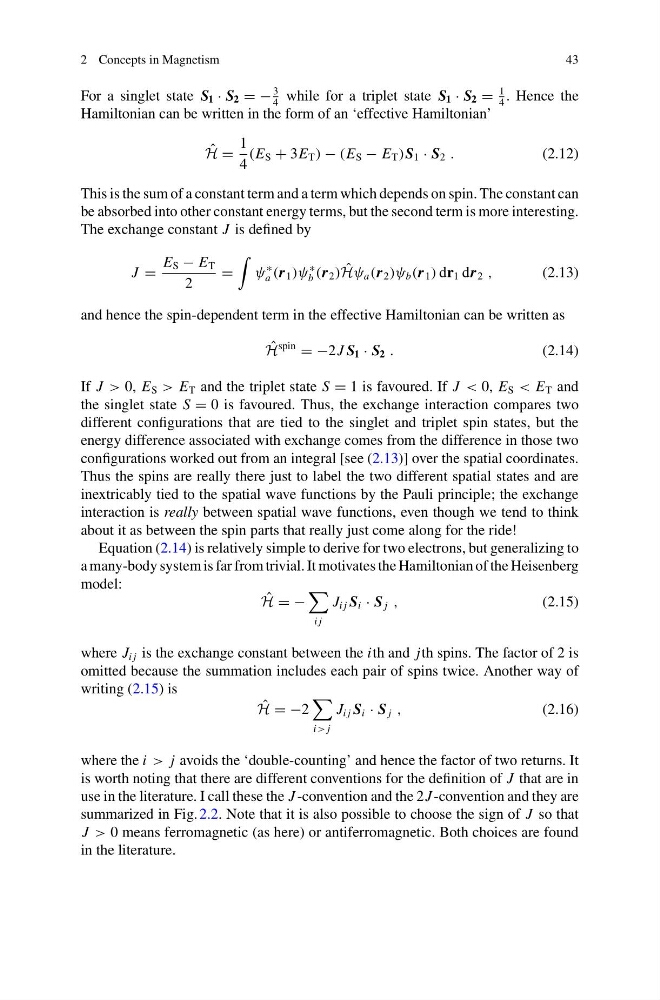
For a singlet state S 1 · S 2 = −
3
4
while for a triplet state S 1 · S 2 =
1
4
. Hence the
Hamiltonian can be written in the form of an ‘effective Hamiltonian’
ˆ
H =
1
4
(E S + 3E T ) − (E S − E T )S 1 · S 2 .
(2.12)
This is the sum of a constant term and a term which depends on spin. The constant can
be absorbed into other constant energy terms, but the second term is more interesting.
The exchange constant J is defined by
J =
E S − E T
2
=
ψ
∗
a (r 1 )ψ
∗
b (r 2 ) ˆ
Hψ a (r 2 )ψ b (r 1 ) dr 1 dr 2 ,
(2.13)
and hence the spin-dependent term in the effective Hamiltonian can be written as
ˆ
H
spin
= −2J S 1 · S 2 .
(2.14)
If J > 0, E S > E T and the triplet state S = 1 is favoured. If J < 0, E S < E T and
the singlet state S = 0 is favoured. Thus, the exchange interaction compares two
different configurations that are tied to the singlet and triplet spin states, but the
energy difference associated with exchange comes from the difference in those two
configurations worked out from an integral [see (2.13)] over the spatial coordinates.
Thus the spins are really there just to label the two different spatial states and are
inextricably tied to the spatial wave functions by the Pauli principle; the exchange
interaction is really between spatial wave functions, even though we tend to think
about it as between the spin parts that really just come along for the ride!
Equation (2.14) is relatively simple to derive for two electrons, but generalizing to
a many-body system is far from trivial. It motivates the Hamiltonian of the Heisenberg
model:
ˆ
H = −
i j
J i j S i · S j ,
(2.15)
where J i j is the exchange constant between the ith and jth spins. The factor of 2 is
omitted because the summation includes each pair of spins twice. Another way of
writing (2.15) is
ˆ
H = −2
i> j
J i j S i · S j ,
(2.16)
where the i > j avoids the ‘double-counting’ and hence the factor of two returns. It
is worth noting that there are different conventions for the definition of J that are in
use in the literature. I call these the J -convention and the 2J -convention and they are
summarized in Fig. 2.2. Note that it is also possible to choose the sign of J so that
J > 0 means ferromagnetic (as here) or antiferromagnetic. Both choices are found
in the literature.
43
For a singlet state S 1 · S 2 = −
3
4
while for a triplet state S 1 · S 2 =
1
4
. Hence the
Hamiltonian can be written in the form of an ‘effective Hamiltonian’
ˆ
H =
1
4
(E S + 3E T ) − (E S − E T )S 1 · S 2 .
(2.12)
This is the sum of a constant term and a term which depends on spin. The constant can
be absorbed into other constant energy terms, but the second term is more interesting.
The exchange constant J is defined by
J =
E S − E T
2
=
ψ
∗
a (r 1 )ψ
∗
b (r 2 ) ˆ
Hψ a (r 2 )ψ b (r 1 ) dr 1 dr 2 ,
(2.13)
and hence the spin-dependent term in the effective Hamiltonian can be written as
ˆ
H
spin
= −2J S 1 · S 2 .
(2.14)
If J > 0, E S > E T and the triplet state S = 1 is favoured. If J < 0, E S < E T and
the singlet state S = 0 is favoured. Thus, the exchange interaction compares two
different configurations that are tied to the singlet and triplet spin states, but the
energy difference associated with exchange comes from the difference in those two
configurations worked out from an integral [see (2.13)] over the spatial coordinates.
Thus the spins are really there just to label the two different spatial states and are
inextricably tied to the spatial wave functions by the Pauli principle; the exchange
interaction is really between spatial wave functions, even though we tend to think
about it as between the spin parts that really just come along for the ride!
Equation (2.14) is relatively simple to derive for two electrons, but generalizing to
a many-body system is far from trivial. It motivates the Hamiltonian of the Heisenberg
model:
ˆ
H = −
i j
J i j S i · S j ,
(2.15)
where J i j is the exchange constant between the ith and jth spins. The factor of 2 is
omitted because the summation includes each pair of spins twice. Another way of
writing (2.15) is
ˆ
H = −2
i> j
J i j S i · S j ,
(2.16)
where the i > j avoids the ‘double-counting’ and hence the factor of two returns. It
is worth noting that there are different conventions for the definition of J that are in
use in the literature. I call these the J -convention and the 2J -convention and they are
summarized in Fig. 2.2. Note that it is also possible to choose the sign of J so that
J > 0 means ferromagnetic (as here) or antiferromagnetic. Both choices are found
in the literature.