

194
J.-P. Brison
d =
1
2ψ
[−
↑
( ˆ
n)(e x + ie y ) +
↓
( ˆ
n)(e x − ie y )] +
0 e z
=
1
2ψ
[(−ζ
↑
z
ˆ
k z )(e x + ie y ) + (ζ
↓
z
ˆ
k z )(e x − ie y )] + (ζ
0
x
ˆ
k x + iζ
0
y
ˆ
k y )e z
=
1
2ψ
ζ
↓
z − ζ
↑
z
ˆ
k z e x − i
ζ
↑
z + ζ
↓
z
ˆ
k z e y + 2
ζ
0
x
ˆ
k x + iζ
0
y
ˆ
k y
e z
.
(6.51)
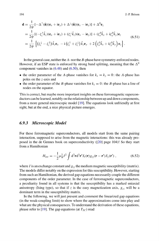
In the general case, neither the A- nor the B-phase have symmetry-enforced nodes.
However, if an ESP state is enforced by strong band splitting, meaning that the
0
component vanishes in (6.48) and (6.50), then
• the order parameter of the A-phase vanishes for k x = k y = 0 : the A-phase has
poles on the z-axis and
• the order parameter of the B-phase vanishes for k z = 0 : the B-phase has a line of
nodes on the equator.
This is correct, but maybe more important insights on these ferromagnetic superconductors can be learned, notably on the relationship between up and down components,
from a more general microscopic model [19]. The equations look unfriendly at first
sight, but at the end, a nice physical picture emerges.
6.9.3 Microscopic Model
For these ferromagnetic superconductors, all models start from the same pairing
interaction, supposed to arise from the magnetic interactions: this was already proposed in the de Gennes book on superconductivity ([20] page 104)! So they start
from a Hamiltonian
H int = −
1
2
μ
2
B I
2
d
3 rd
3 r
S i (r)χ i j (r − r
)S j (r
) ,
(6.52)
where I is an exchange constant and χ i j the medium magnetic susceptibility (matrix).
The models differ notably on the expression for this susceptibility. However, starting
from such an Hamiltonian, the derived gap equations necessarily couple the different
components of the order parameter. In the case of ferromagnetic superconductors,
a peculiarity found in all systems is that the susceptibility has a marked uniaxial
anisotropy (Ising type), so that if z is the easy magnetization axis, χ zz will be a
dominant term in the susceptibility matrix.
In the following, we will just present and comment the linearized gap equations
(in the weak-coupling limit) to show where the approximations come into play and
what are the physical consequences. To understand the derivation of these equations,
please refer to [19]. The gap equations (at T SC ) read
J.-P. Brison
d =
1
2ψ
[−
↑
( ˆ
n)(e x + ie y ) +
↓
( ˆ
n)(e x − ie y )] +
0 e z
=
1
2ψ
[(−ζ
↑
z
ˆ
k z )(e x + ie y ) + (ζ
↓
z
ˆ
k z )(e x − ie y )] + (ζ
0
x
ˆ
k x + iζ
0
y
ˆ
k y )e z
=
1
2ψ
ζ
↓
z − ζ
↑
z
ˆ
k z e x − i
ζ
↑
z + ζ
↓
z
ˆ
k z e y + 2
ζ
0
x
ˆ
k x + iζ
0
y
ˆ
k y
e z
.
(6.51)
In the general case, neither the A- nor the B-phase have symmetry-enforced nodes.
However, if an ESP state is enforced by strong band splitting, meaning that the
0
component vanishes in (6.48) and (6.50), then
• the order parameter of the A-phase vanishes for k x = k y = 0 : the A-phase has
poles on the z-axis and
• the order parameter of the B-phase vanishes for k z = 0 : the B-phase has a line of
nodes on the equator.
This is correct, but maybe more important insights on these ferromagnetic superconductors can be learned, notably on the relationship between up and down components,
from a more general microscopic model [19]. The equations look unfriendly at first
sight, but at the end, a nice physical picture emerges.
6.9.3 Microscopic Model
For these ferromagnetic superconductors, all models start from the same pairing
interaction, supposed to arise from the magnetic interactions: this was already proposed in the de Gennes book on superconductivity ([20] page 104)! So they start
from a Hamiltonian
H int = −
1
2
μ
2
B I
2
d
3 rd
3 r
S i (r)χ i j (r − r
)S j (r
) ,
(6.52)
where I is an exchange constant and χ i j the medium magnetic susceptibility (matrix).
The models differ notably on the expression for this susceptibility. However, starting
from such an Hamiltonian, the derived gap equations necessarily couple the different
components of the order parameter. In the case of ferromagnetic superconductors,
a peculiarity found in all systems is that the susceptibility has a marked uniaxial
anisotropy (Ising type), so that if z is the easy magnetization axis, χ zz will be a
dominant term in the susceptibility matrix.
In the following, we will just present and comment the linearized gap equations
(in the weak-coupling limit) to show where the approximations come into play and
what are the physical consequences. To understand the derivation of these equations,
please refer to [19]. The gap equations (at T SC ) read