

38
H. Vallen
-30
-25
-20
-15
-10
-5
0
5
10
0
50 100 150 200 250 300 350 400 450 500 550 600 650 700 750 800 850 900 950 1000
dB
kHz
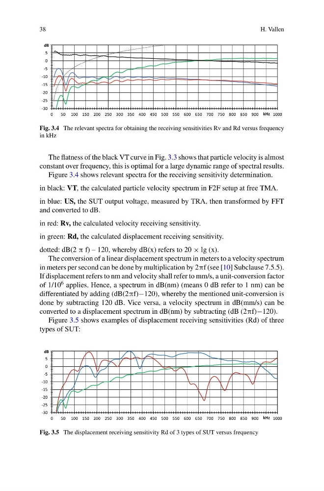
Fig. 3.4 The relevant spectra for obtaining the receiving sensitivities Rv and Rd versus frequency
in kHz
The flatness of the black VT curve in Fig. 3.3 shows that particle velocity is almost
constant over frequency, this is optimal for a large dynamic range of spectral results.
Figure 3.4 shows relevant spectra for the receiving sensitivity determination.
in black: VT, the calculated particle velocity spectrum in F2F setup at free TMA.
in blue: US, the SUT output voltage, measured by TRA, then transformed by FFT
and converted to dB.
in red: Rv, the calculated velocity receiving sensitivity.
in green: Rd, the calculated displacement receiving sensitivity.
dotted: dB(2 π f) – 120, whereby dB(x) refers to 20 × lg (x).
The conversion of a linear displacement spectrum in meters to a velocity spectrum
in meters per second can be done by multiplication by 2πf (see [10] Subclause 7.5.5).
If displacement refers to nm and velocity shall refer to mm/s, a unit-conversion factor
of 1/10
6 applies. Hence, a spectrum in dB(nm) (means 0 dB refer to 1 nm) can be
differentiated by adding (dB(2πf)−120), whereby the mentioned unit-conversion is
done by subtracting 120 dB. Vice versa, a velocity spectrum in dB(mm/s) can be
converted to a displacement spectrum in dB(nm) by subtracting (dB (2πf)−120).
Figure 3.5 shows examples of displacement receiving sensitivities (Rd) of three
types of SUT:
-30
-25
-20
-15
-10
-5
0
5
10
0
50 100 150 200 250 300 350 400 450 500 550 600 650 700 750 800 850 900 950 1000
dB
kHz
Fig. 3.5 The displacement receiving sensitivity Rd of 3 types of SUT versus frequency
H. Vallen
-30
-25
-20
-15
-10
-5
0
5
10
0
50 100 150 200 250 300 350 400 450 500 550 600 650 700 750 800 850 900 950 1000
dB
kHz
Fig. 3.4 The relevant spectra for obtaining the receiving sensitivities Rv and Rd versus frequency
in kHz
The flatness of the black VT curve in Fig. 3.3 shows that particle velocity is almost
constant over frequency, this is optimal for a large dynamic range of spectral results.
Figure 3.4 shows relevant spectra for the receiving sensitivity determination.
in black: VT, the calculated particle velocity spectrum in F2F setup at free TMA.
in blue: US, the SUT output voltage, measured by TRA, then transformed by FFT
and converted to dB.
in red: Rv, the calculated velocity receiving sensitivity.
in green: Rd, the calculated displacement receiving sensitivity.
dotted: dB(2 π f) – 120, whereby dB(x) refers to 20 × lg (x).
The conversion of a linear displacement spectrum in meters to a velocity spectrum
in meters per second can be done by multiplication by 2πf (see [10] Subclause 7.5.5).
If displacement refers to nm and velocity shall refer to mm/s, a unit-conversion factor
of 1/10
6 applies. Hence, a spectrum in dB(nm) (means 0 dB refer to 1 nm) can be
differentiated by adding (dB(2πf)−120), whereby the mentioned unit-conversion is
done by subtracting 120 dB. Vice versa, a velocity spectrum in dB(mm/s) can be
converted to a displacement spectrum in dB(nm) by subtracting (dB (2πf)−120).
Figure 3.5 shows examples of displacement receiving sensitivities (Rd) of three
types of SUT:
-30
-25
-20
-15
-10
-5
0
5
10
0
50 100 150 200 250 300 350 400 450 500 550 600 650 700 750 800 850 900 950 1000
dB
kHz
Fig. 3.5 The displacement receiving sensitivity Rd of 3 types of SUT versus frequency