

484
K. Zhang et al.
(x i − x 0 )
2
+(y i − y 0 )
2
=c
2
(t i − t 0 )
2
(42.7)
Consider the predicted location are (x, y), then the predicted impact time t
0 can
be calculated as
t
0 (x, y) = t i −
(x i − x) 2 +(y i − y)
2
c
(42.8)
For each sensors, the impact time t 0 should be the same, it is mean that for the
true impact location (x 0 , y 0 )
t 0 (x 0 , y 0 ) = t i −
(x i − x 0 ) 2 +(y i − y 0 )
2
c
(42.9)
When (x, y) take other value, t
0 would not be the same. Then the error function
E(x 0 ,y 0 ) can be defined as
E(x 0 , y 0 ) =
N
i=1
(t i −
(x i − x 0 ) 2 +(y i − y 0 )
2
c
− ˜
t 0 )
2
(42.10)
The variable ˜
t 0 is the arithmetic mean of t 0 . Ideally, for the correct values of (x 0 ,
y 0 ), the error function should give a zero value. Therefore, we need to minimize the
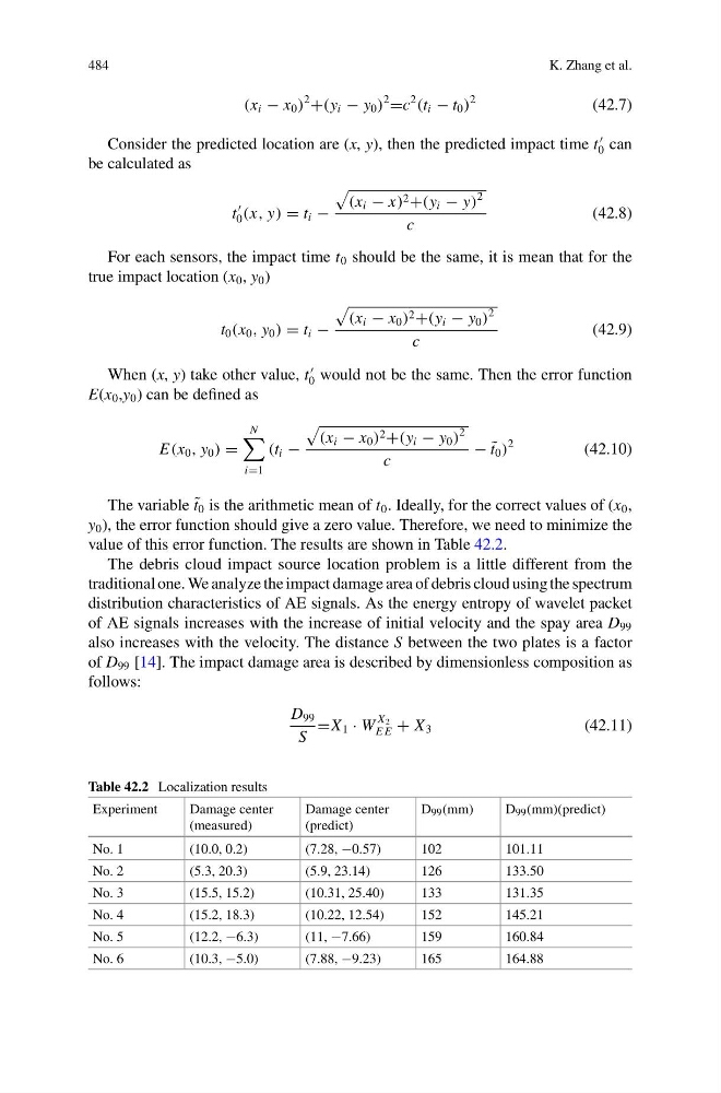
value of this error function. The results are shown in Table 42.2.
The debris cloud impact source location problem is a little different from the
traditional one. We analyze the impact damage area of debris cloud using the spectrum
distribution characteristics of AE signals. As the energy entropy of wavelet packet
of AE signals increases with the increase of initial velocity and the spay area D 99
also increases with the velocity. The distance S between the two plates is a factor
of D 99 [14]. The impact damage area is described by dimensionless composition as
follows:
D 99
S
=X 1 · W
X 2
E E + X 3
(42.11)
Table 42.2 Localization results
Experiment
Damage center
(measured)
Damage center
(predict)
D 99 (mm)
D 99 (mm)(predict)
No. 1
(10.0, 0.2)
(7.28, −0.57)
102
101.11
No. 2
(5.3, 20.3)
(5.9, 23.14)
126
133.50
No. 3
(15.5, 15.2)
(10.31, 25.40)
133
131.35
No. 4
(15.2, 18.3)
(10.22, 12.54)
152
145.21
No. 5
(12.2, −6.3)
(11, −7.66)
159
160.84
No. 6
(10.3, −5.0)
(7.88, −9.23)
165
164.88
K. Zhang et al.
(x i − x 0 )
2
+(y i − y 0 )
2
=c
2
(t i − t 0 )
2
(42.7)
Consider the predicted location are (x, y), then the predicted impact time t
0 can
be calculated as
t
0 (x, y) = t i −
(x i − x) 2 +(y i − y)
2
c
(42.8)
For each sensors, the impact time t 0 should be the same, it is mean that for the
true impact location (x 0 , y 0 )
t 0 (x 0 , y 0 ) = t i −
(x i − x 0 ) 2 +(y i − y 0 )
2
c
(42.9)
When (x, y) take other value, t
0 would not be the same. Then the error function
E(x 0 ,y 0 ) can be defined as
E(x 0 , y 0 ) =
N
i=1
(t i −
(x i − x 0 ) 2 +(y i − y 0 )
2
c
− ˜
t 0 )
2
(42.10)
The variable ˜
t 0 is the arithmetic mean of t 0 . Ideally, for the correct values of (x 0 ,
y 0 ), the error function should give a zero value. Therefore, we need to minimize the
value of this error function. The results are shown in Table 42.2.
The debris cloud impact source location problem is a little different from the
traditional one. We analyze the impact damage area of debris cloud using the spectrum
distribution characteristics of AE signals. As the energy entropy of wavelet packet
of AE signals increases with the increase of initial velocity and the spay area D 99
also increases with the velocity. The distance S between the two plates is a factor
of D 99 [14]. The impact damage area is described by dimensionless composition as
follows:
D 99
S
=X 1 · W
X 2
E E + X 3
(42.11)
Table 42.2 Localization results
Experiment
Damage center
(measured)
Damage center
(predict)
D 99 (mm)
D 99 (mm)(predict)
No. 1
(10.0, 0.2)
(7.28, −0.57)
102
101.11
No. 2
(5.3, 20.3)
(5.9, 23.14)
126
133.50
No. 3
(15.5, 15.2)
(10.31, 25.40)
133
131.35
No. 4
(15.2, 18.3)
(10.22, 12.54)
152
145.21
No. 5
(12.2, −6.3)
(11, −7.66)
159
160.84
No. 6
(10.3, −5.0)
(7.88, −9.23)
165
164.88