

42 Damage Localization of Debris Cloud Hypervelocity Impact …
483
42.4 Debris Cloud Impact Localization
In this paper, the projectile impacts the double-layer plate structure normally. In
this condition, the damage on the rear plate is symmetrical. The signals received by
sensors may be from the impact damage center, or from the damage boundary, or
between them. It is difficult to confirm where the first arrival signals from. But due
to the symmetry of debris cloud structure as shown in Fig. 42.2, the location should
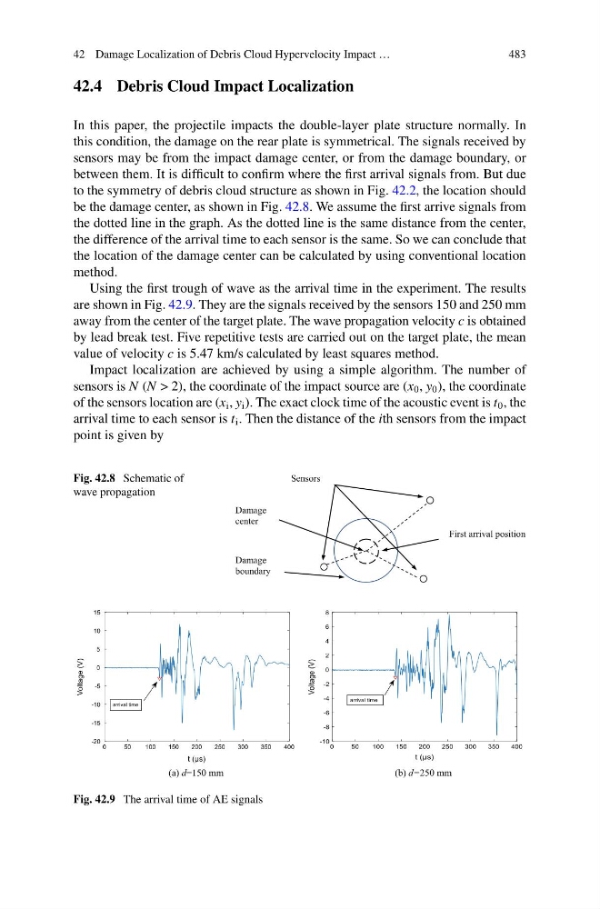
be the damage center, as shown in Fig. 42.8. We assume the first arrive signals from
the dotted line in the graph. As the dotted line is the same distance from the center,
the difference of the arrival time to each sensor is the same. So we can conclude that
the location of the damage center can be calculated by using conventional location
method.
Using the first trough of wave as the arrival time in the experiment. The results
are shown in Fig. 42.9. They are the signals received by the sensors 150 and 250 mm
away from the center of the target plate. The wave propagation velocity c is obtained
by lead break test. Five repetitive tests are carried out on the target plate, the mean
value of velocity c is 5.47 km/s calculated by least squares method.
Impact localization are achieved by using a simple algorithm. The number of
sensors is N (N > 2), the coordinate of the impact source are (x 0 , y 0 ), the coordinate
of the sensors location are (x i , y i ). The exact clock time of the acoustic event is t 0 , the
arrival time to each sensor is t i . Then the distance of the ith sensors from the impact
point is given by
Fig. 42.8 Schematic of
wave propagation
First arrival position
Sensors
Damage
boundary
Damage
center
(a) d=150 mm
(b) d=250 mm
Fig. 42.9 The arrival time of AE signals
483
42.4 Debris Cloud Impact Localization
In this paper, the projectile impacts the double-layer plate structure normally. In
this condition, the damage on the rear plate is symmetrical. The signals received by
sensors may be from the impact damage center, or from the damage boundary, or
between them. It is difficult to confirm where the first arrival signals from. But due
to the symmetry of debris cloud structure as shown in Fig. 42.2, the location should
be the damage center, as shown in Fig. 42.8. We assume the first arrive signals from
the dotted line in the graph. As the dotted line is the same distance from the center,
the difference of the arrival time to each sensor is the same. So we can conclude that
the location of the damage center can be calculated by using conventional location
method.
Using the first trough of wave as the arrival time in the experiment. The results
are shown in Fig. 42.9. They are the signals received by the sensors 150 and 250 mm
away from the center of the target plate. The wave propagation velocity c is obtained
by lead break test. Five repetitive tests are carried out on the target plate, the mean
value of velocity c is 5.47 km/s calculated by least squares method.
Impact localization are achieved by using a simple algorithm. The number of
sensors is N (N > 2), the coordinate of the impact source are (x 0 , y 0 ), the coordinate
of the sensors location are (x i , y i ). The exact clock time of the acoustic event is t 0 , the
arrival time to each sensor is t i . Then the distance of the ith sensors from the impact
point is given by
Fig. 42.8 Schematic of
wave propagation
First arrival position
Sensors
Damage
boundary
Damage
center
(a) d=150 mm
(b) d=250 mm
Fig. 42.9 The arrival time of AE signals