

37 A Method of Vacuum Leak Detecting Based on Acoustic Emission …
423
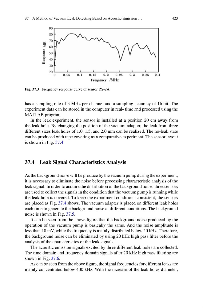
Fig. 37.3 Frequency response curve of sensor RS-2A
has a sampling rate of 3 MHz per channel and a sampling accuracy of 16 bit. The
experiment data can be stored in the computer in real- time and processed using the
MATLAB program.
In the leak experiment, the sensor is installed at a position 20 cm away from
the leak hole. By changing the position of the vacuum adapter, the leak from three
different sizes leak holes of 1.0, 1.5, and 2.0 mm can be realized. The no-leak state
can be produced with tape covering as a comparative experiment. The sensor layout
is shown in Fig. 37.4.
37.4 Leak Signal Characteristics Analysis
As the background noise will be produce by the vacuum pump during the experiment,
it is necessary to eliminate the noise before processing characteristic analysis of the
leak signal. In order to acquire the distribution of the background noise, three sensors
are used to collect the signals in the condition that the vacuum pump is running while
the leak hole is covered. To keep the experiment conditions consistent, the sensors
are placed as Fig. 37.4 shows. The vacuum adapter is placed on different leak holes
each time to generate the background noise at different conditions. The background
noise is shown in Fig. 37.5.
It can be seen from the above figure that the background noise produced by the
operation of the vacuum pump is basically the same. And the noise amplitude is
less than 10 mV, while the frequency is mainly distributed below 20 kHz. Therefore,
the background noise can be eliminated by using 20 kHz high pass filter before the
analysis of the characteristics of the leak signals.
The acoustic emission signals excited by three different leak holes are collected.
The time domain and frequency domain signals after 20 kHz high pass filtering are
shown in Fig. 37.6.
As can be seen from the above figure, the signal frequencies for different leaks are
mainly concentrated below 400 kHz. With the increase of the leak holes diameter,
423
Fig. 37.3 Frequency response curve of sensor RS-2A
has a sampling rate of 3 MHz per channel and a sampling accuracy of 16 bit. The
experiment data can be stored in the computer in real- time and processed using the
MATLAB program.
In the leak experiment, the sensor is installed at a position 20 cm away from
the leak hole. By changing the position of the vacuum adapter, the leak from three
different sizes leak holes of 1.0, 1.5, and 2.0 mm can be realized. The no-leak state
can be produced with tape covering as a comparative experiment. The sensor layout
is shown in Fig. 37.4.
37.4 Leak Signal Characteristics Analysis
As the background noise will be produce by the vacuum pump during the experiment,
it is necessary to eliminate the noise before processing characteristic analysis of the
leak signal. In order to acquire the distribution of the background noise, three sensors
are used to collect the signals in the condition that the vacuum pump is running while
the leak hole is covered. To keep the experiment conditions consistent, the sensors
are placed as Fig. 37.4 shows. The vacuum adapter is placed on different leak holes
each time to generate the background noise at different conditions. The background
noise is shown in Fig. 37.5.
It can be seen from the above figure that the background noise produced by the
operation of the vacuum pump is basically the same. And the noise amplitude is
less than 10 mV, while the frequency is mainly distributed below 20 kHz. Therefore,
the background noise can be eliminated by using 20 kHz high pass filter before the
analysis of the characteristics of the leak signals.
The acoustic emission signals excited by three different leak holes are collected.
The time domain and frequency domain signals after 20 kHz high pass filtering are
shown in Fig. 37.6.
As can be seen from the above figure, the signal frequencies for different leaks are
mainly concentrated below 400 kHz. With the increase of the leak holes diameter,