

27 Evaluation of Fatigue Damage in RC Slabs Considering Water Infiltration …
327
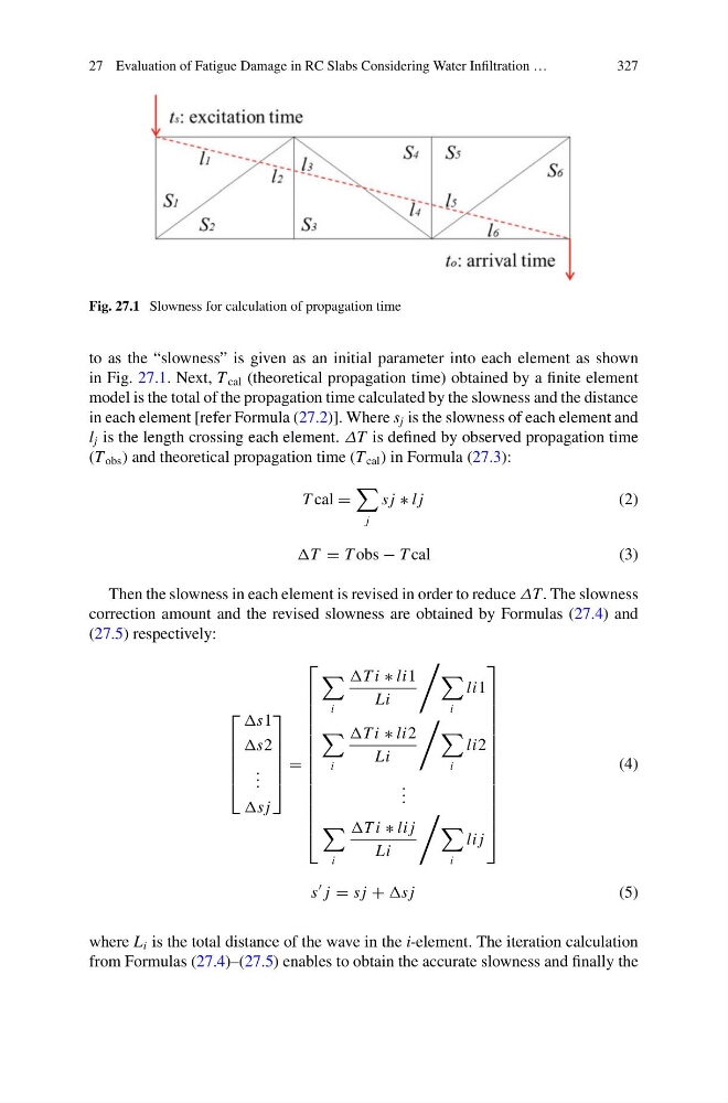
Fig. 27.1 Slowness for calculation of propagation time
to as the “slowness” is given as an initial parameter into each element as shown
in Fig. 27.1. Next, T cal (theoretical propagation time) obtained by a finite element
model is the total of the propagation time calculated by the slowness and the distance
in each element [refer Formula (27.2)]. Where s j is the slowness of each element and
l j is the length crossing each element. ΔT is defined by observed propagation time
(T obs ) and theoretical propagation time (T cal ) in Formula (27.3):
T cal =
j
s j ∗ l j
(2)
T = T obs − T cal
(3)
Then the slowness in each element is revised in order to reduce ΔT. The slowness
correction amount and the revised slowness are obtained by Formulas (27.4) and
(27.5) respectively:
⎡
⎢
⎢
⎢
⎢
⎣
s1
s2
. . .
s j
⎤
⎥
⎥
⎥
⎥
⎦
=
⎡
⎢
⎢
⎢
⎢
⎢
⎢
⎢
⎢
⎢
⎢
⎢
⎢
⎢
⎢
⎣
i
T i ∗ li1
Li
i
li1
i
T i ∗ li2
Li
i
li2
. . .
i
T i ∗ li j
Li
i
li j
⎤
⎥
⎥
⎥
⎥
⎥
⎥
⎥
⎥
⎥
⎥
⎥
⎥
⎥
⎥
⎦
(4)
s
j = s j + s j
(5)
where L i is the total distance of the wave in the i-element. The iteration calculation
from Formulas (27.4)–(27.5) enables to obtain the accurate slowness and finally the
327
Fig. 27.1 Slowness for calculation of propagation time
to as the “slowness” is given as an initial parameter into each element as shown
in Fig. 27.1. Next, T cal (theoretical propagation time) obtained by a finite element
model is the total of the propagation time calculated by the slowness and the distance
in each element [refer Formula (27.2)]. Where s j is the slowness of each element and
l j is the length crossing each element. ΔT is defined by observed propagation time
(T obs ) and theoretical propagation time (T cal ) in Formula (27.3):
T cal =
j
s j ∗ l j
(2)
T = T obs − T cal
(3)
Then the slowness in each element is revised in order to reduce ΔT. The slowness
correction amount and the revised slowness are obtained by Formulas (27.4) and
(27.5) respectively:
⎡
⎢
⎢
⎢
⎢
⎣
s1
s2
. . .
s j
⎤
⎥
⎥
⎥
⎥
⎦
=
⎡
⎢
⎢
⎢
⎢
⎢
⎢
⎢
⎢
⎢
⎢
⎢
⎢
⎢
⎢
⎣
i
T i ∗ li1
Li
i
li1
i
T i ∗ li2
Li
i
li2
. . .
i
T i ∗ li j
Li
i
li j
⎤
⎥
⎥
⎥
⎥
⎥
⎥
⎥
⎥
⎥
⎥
⎥
⎥
⎥
⎥
⎦
(4)
s
j = s j + s j
(5)
where L i is the total distance of the wave in the i-element. The iteration calculation
from Formulas (27.4)–(27.5) enables to obtain the accurate slowness and finally the