

320
Y. Yang et al.
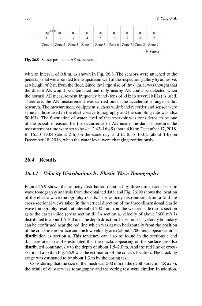
Fig. 26.8 Sensor position in AE measurement
with an interval of 0.8 m, as shown in Fig. 26.8. The sensors were attached to the
pedestals that were bonded to the upstream wall of the inspection gallery by adhesive,
at a height of 2 m from the floor. Since the large size of the dam, it was thought that
the distant AE would be attenuated and only nearby AE could be detected when
the normal AE measurement frequency band (tens of kHz to several MHz) is used.
Therefore, the AE measurement was carried out in the acceleration range in this
research. The measurement equipment such as wide band recorder and sensor were
same as those used in the elastic wave tomography and the sampling rate was also
50 kHz. The fluctuation of water level of the reservoir was considered to be one
of the possible reasons for the occurrence of AE inside the dam. Therefore, the
measurement time were set to be A: 12:43–16:45 (about 4 h) on December 17, 2018,
B: 16:50–19:04 (about 2 h) on the same day, and C: 8:55–13:02 (about 4 h) on
December 18, 2018, when the water level were changing continuously.
26.4 Results
26.4.1 Velocity Distributions by Elastic Wave Tomography
Figure 26.9 shows the velocity distribution obtained by three-dimensional elastic
wave tomography analysis from the obtained data, and Fig. 26.10 shows the location
of the elastic wave tomography results. The velocity distributions from a to d are
cross-sectional views taken in the vertical direction of the three-dimensional elastic
wave tomography result, at interval of 200 mm from the western side (cross section
a) to the eastern side (cross section d). In section a, velocity of about 3600 m/s is
distributed to about 1.5–2.0 m in the depth direction. In section b, a velocity boundary
can be confirmed near the red line which was drawn horizontally from the position
of the crack in the surface and the low velocity area (about 3700 m/s) appears similar
distribution as section a. This tendency can also be found in the sections c and
d. Therefore, it can be estimated that the cracks appearing on the surface are also
distributed continuously to the depth of about 1.5–2.0 m. And the red line of crosssectional a to d in Fig. 26.9 was the estimation of the crack’s location. The cracking
range was estimated to be about 1.3 m by the coring test.
Considering that the size of the mesh was 500 mm in the depth direction (Z axis),
the result of elastic wave tomography and the coring test were similar. In addition,
Y. Yang et al.
Fig. 26.8 Sensor position in AE measurement
with an interval of 0.8 m, as shown in Fig. 26.8. The sensors were attached to the
pedestals that were bonded to the upstream wall of the inspection gallery by adhesive,
at a height of 2 m from the floor. Since the large size of the dam, it was thought that
the distant AE would be attenuated and only nearby AE could be detected when
the normal AE measurement frequency band (tens of kHz to several MHz) is used.
Therefore, the AE measurement was carried out in the acceleration range in this
research. The measurement equipment such as wide band recorder and sensor were
same as those used in the elastic wave tomography and the sampling rate was also
50 kHz. The fluctuation of water level of the reservoir was considered to be one
of the possible reasons for the occurrence of AE inside the dam. Therefore, the
measurement time were set to be A: 12:43–16:45 (about 4 h) on December 17, 2018,
B: 16:50–19:04 (about 2 h) on the same day, and C: 8:55–13:02 (about 4 h) on
December 18, 2018, when the water level were changing continuously.
26.4 Results
26.4.1 Velocity Distributions by Elastic Wave Tomography
Figure 26.9 shows the velocity distribution obtained by three-dimensional elastic
wave tomography analysis from the obtained data, and Fig. 26.10 shows the location
of the elastic wave tomography results. The velocity distributions from a to d are
cross-sectional views taken in the vertical direction of the three-dimensional elastic
wave tomography result, at interval of 200 mm from the western side (cross section
a) to the eastern side (cross section d). In section a, velocity of about 3600 m/s is
distributed to about 1.5–2.0 m in the depth direction. In section b, a velocity boundary
can be confirmed near the red line which was drawn horizontally from the position
of the crack in the surface and the low velocity area (about 3700 m/s) appears similar
distribution as section a. This tendency can also be found in the sections c and
d. Therefore, it can be estimated that the cracks appearing on the surface are also
distributed continuously to the depth of about 1.5–2.0 m. And the red line of crosssectional a to d in Fig. 26.9 was the estimation of the crack’s location. The cracking
range was estimated to be about 1.3 m by the coring test.
Considering that the size of the mesh was 500 mm in the depth direction (Z axis),
the result of elastic wave tomography and the coring test were similar. In addition,