

10 Prediction of Residual Life of Oil and Gas Pipeline Corrosion …
111
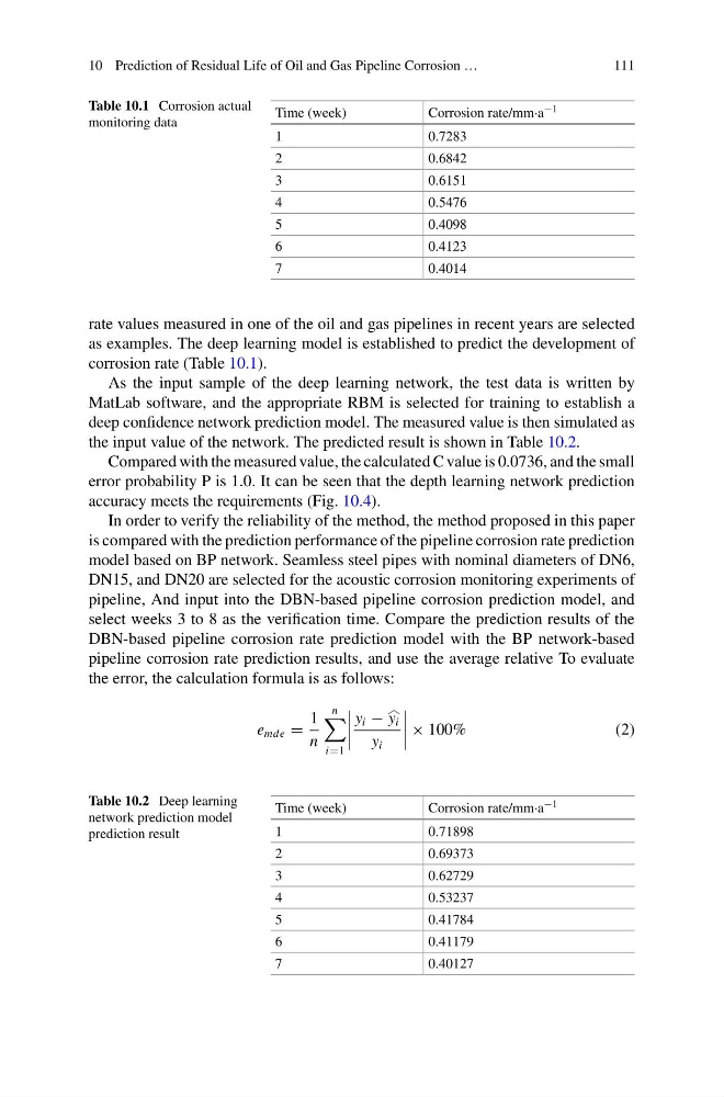
Table 10.1 Corrosion actual
monitoring data
Time (week)
Corrosion rate/mm·a −1
1
0.7283
2
0.6842
3
0.6151
4
0.5476
5
0.4098
6
0.4123
7
0.4014
rate values measured in one of the oil and gas pipelines in recent years are selected
as examples. The deep learning model is established to predict the development of
corrosion rate (Table 10.1).
As the input sample of the deep learning network, the test data is written by
MatLab software, and the appropriate RBM is selected for training to establish a
deep confidence network prediction model. The measured value is then simulated as
the input value of the network. The predicted result is shown in Table 10.2.
Compared with the measured value, the calculated C value is 0.0736, and the small
error probability P is 1.0. It can be seen that the depth learning network prediction
accuracy meets the requirements (Fig. 10.4).
In order to verify the reliability of the method, the method proposed in this paper
is compared with the prediction performance of the pipeline corrosion rate prediction
model based on BP network. Seamless steel pipes with nominal diameters of DN6,
DN15, and DN20 are selected for the acoustic corrosion monitoring experiments of
pipeline, And input into the DBN-based pipeline corrosion prediction model, and
select weeks 3 to 8 as the verification time. Compare the prediction results of the
DBN-based pipeline corrosion rate prediction model with the BP network-based
pipeline corrosion rate prediction results, and use the average relative To evaluate
the error, the calculation formula is as follows:
e mde =
1
n
n
i=1
y i − y i
y i
× 100%
(2)
Table 10.2 Deep learning
network prediction model
prediction result
Time (week)
Corrosion rate/mm·a −1
1
0.71898
2
0.69373
3
0.62729
4
0.53237
5
0.41784
6
0.41179
7
0.40127
111
Table 10.1 Corrosion actual
monitoring data
Time (week)
Corrosion rate/mm·a −1
1
0.7283
2
0.6842
3
0.6151
4
0.5476
5
0.4098
6
0.4123
7
0.4014
rate values measured in one of the oil and gas pipelines in recent years are selected
as examples. The deep learning model is established to predict the development of
corrosion rate (Table 10.1).
As the input sample of the deep learning network, the test data is written by
MatLab software, and the appropriate RBM is selected for training to establish a
deep confidence network prediction model. The measured value is then simulated as
the input value of the network. The predicted result is shown in Table 10.2.
Compared with the measured value, the calculated C value is 0.0736, and the small
error probability P is 1.0. It can be seen that the depth learning network prediction
accuracy meets the requirements (Fig. 10.4).
In order to verify the reliability of the method, the method proposed in this paper
is compared with the prediction performance of the pipeline corrosion rate prediction
model based on BP network. Seamless steel pipes with nominal diameters of DN6,
DN15, and DN20 are selected for the acoustic corrosion monitoring experiments of
pipeline, And input into the DBN-based pipeline corrosion prediction model, and
select weeks 3 to 8 as the verification time. Compare the prediction results of the
DBN-based pipeline corrosion rate prediction model with the BP network-based
pipeline corrosion rate prediction results, and use the average relative To evaluate
the error, the calculation formula is as follows:
e mde =
1
n
n
i=1
y i − y i
y i
× 100%
(2)
Table 10.2 Deep learning
network prediction model
prediction result
Time (week)
Corrosion rate/mm·a −1
1
0.71898
2
0.69373
3
0.62729
4
0.53237
5
0.41784
6
0.41179
7
0.40127