

8 Acoustic Emission and Dual-Tree Complex Wavelet Transform …
85
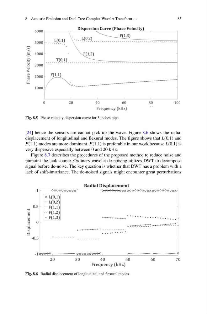
Fig. 8.5 Phase velocity dispersion curve for 3 inches pipe
[24] hence the sensors are cannot pick up the wave. Figure 8.6 shows the radial
displacement of longitudinal and flexural modes. The figure shows that L(0,1) and
F(1,1) modes are more dominant. F(1,1) is preferable in our work because L(0,1) is
very dispersive especially between 0 and 20 kHz.
Figure 8.7 describes the procedures of the proposed method to reduce noise and
pinpoint the leak source. Ordinary wavelet de-noising utilizes DWT to decompose
signal before de-noise. The key question is whether that DWT has a problem with a
lack of shift-invariance. The de-noised signals might encounter great perturbations
Fig. 8.6 Radial displacement of longitudinal and flexural modes
85
Fig. 8.5 Phase velocity dispersion curve for 3 inches pipe
[24] hence the sensors are cannot pick up the wave. Figure 8.6 shows the radial
displacement of longitudinal and flexural modes. The figure shows that L(0,1) and
F(1,1) modes are more dominant. F(1,1) is preferable in our work because L(0,1) is
very dispersive especially between 0 and 20 kHz.
Figure 8.7 describes the procedures of the proposed method to reduce noise and
pinpoint the leak source. Ordinary wavelet de-noising utilizes DWT to decompose
signal before de-noise. The key question is whether that DWT has a problem with a
lack of shift-invariance. The de-noised signals might encounter great perturbations
Fig. 8.6 Radial displacement of longitudinal and flexural modes